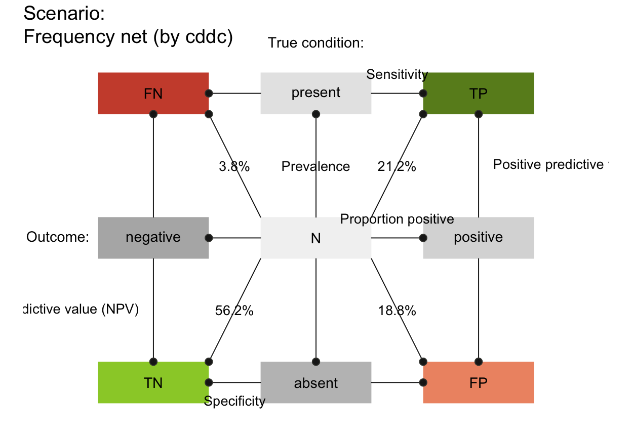
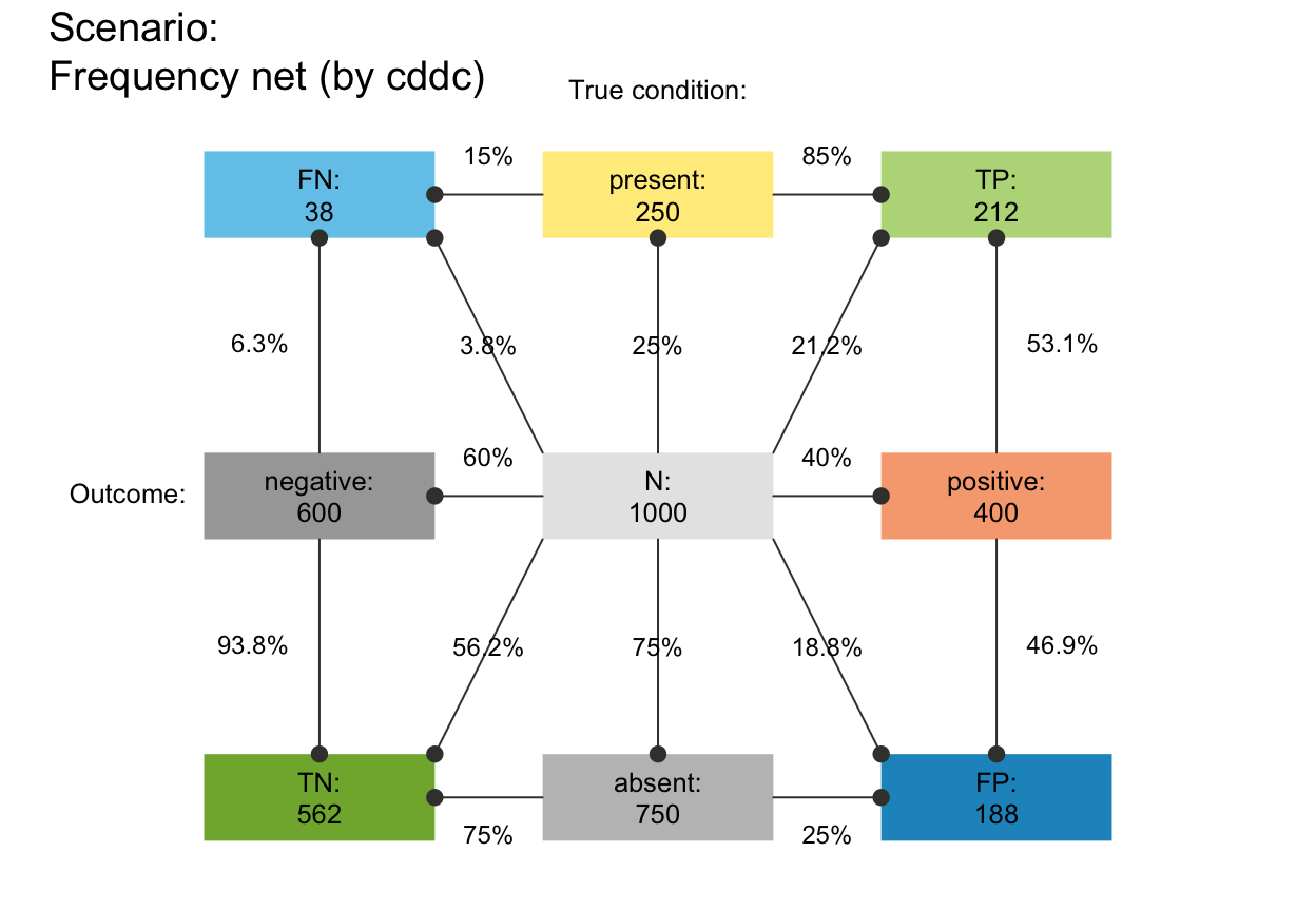
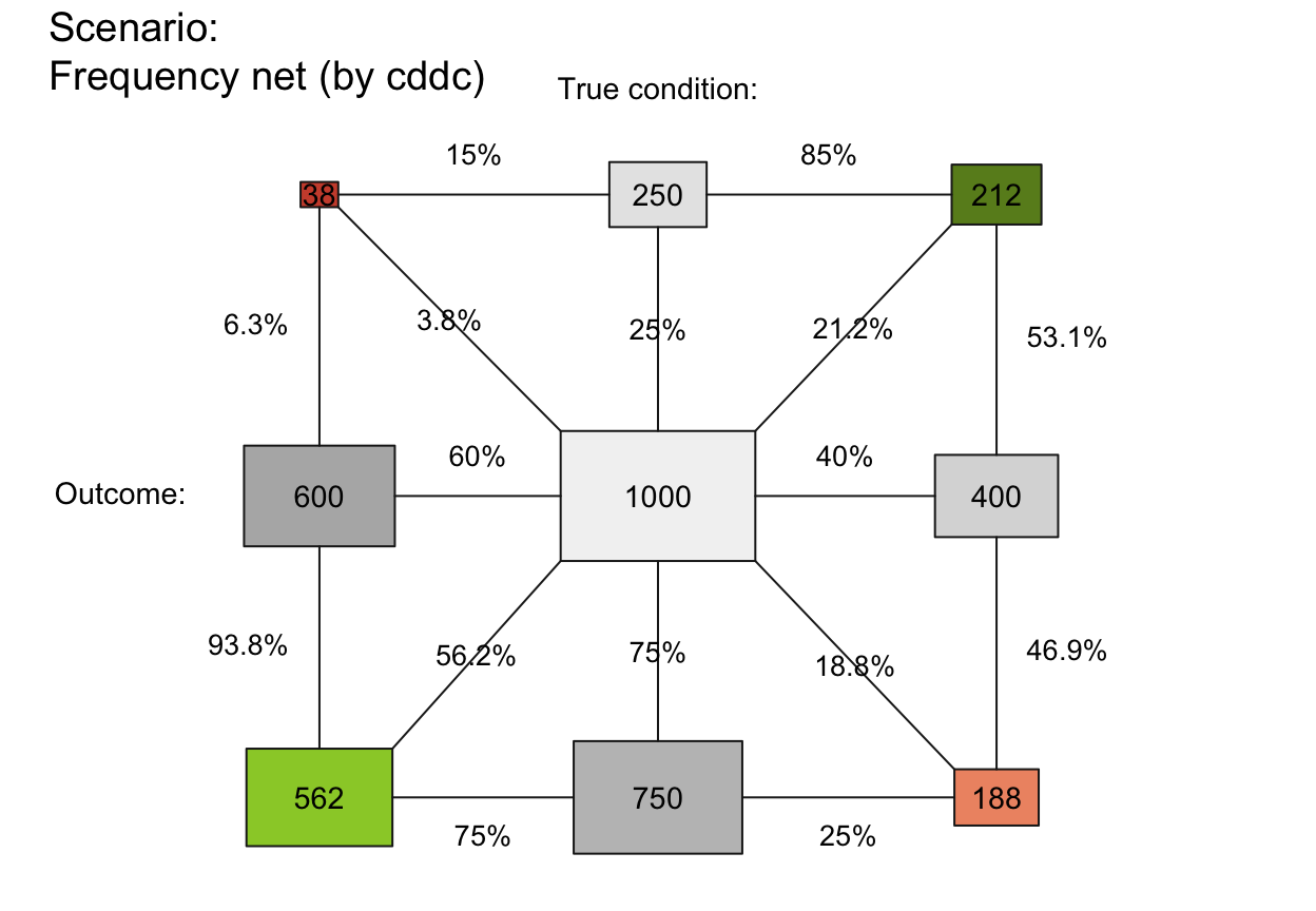
plot_fnet plots a frequency net of
from a sufficient and valid set of 3 essential probabilities
(prev, and
sens or its complement mirt, and
spec or its complement fart)
or existing frequency information freq
and a population size of N individuals.
Usage
plot_fnet(
  prev = num$prev,
  sens = num$sens,
  mirt = NA,
  spec = num$spec,
  fart = NA,
  N = num$N,
  by = "cddc",
  area = "no",
  scale = "p",
  round = TRUE,
  sample = FALSE,
  f_lbl = "num",
  f_lbl_sep = NA,
  f_lwd = 0,
  p_lwd = 1,
  p_scale = FALSE,
  p_lbl = "mix",
  arr_c = NA,
  joint_p = TRUE,
  lbl_txt = txt,
  main = txt$scen_lbl,
  sub = "type",
  title_lbl = NULL,
  cex_lbl = 0.9,
  cex_p_lbl = NA,
  col_pal = pal,
  mar_notes = FALSE,
  ...
)
Source
Binder, K., Krauss, S., and Wiesner, P. (2020). A new visualization for probabilistic situations containing two binary events: The frequency net. Frontiers in Psychology, 11, 750. doi: 10.3389/fpsyg.2020.00750
Arguments
- prev
The condition's prevalence
prev(i.e., the probability of condition beingTRUE).- sens
The decision's sensitivity
sens(i.e., the conditional probability of a positive decision provided that the condition isTRUE).sensis optional when its complementmirtis provided.- mirt
The decision's miss rate
mirt(i.e., the conditional probability of a negative decision provided that the condition isTRUE).mirtis optional when its complementsensis provided.- spec
The decision's specificity value
spec(i.e., the conditional probability of a negative decision provided that the condition isFALSE).specis optional when its complementfartis provided.- fart
The decision's false alarm rate
fart(i.e., the conditional probability of a positive decision provided that the condition isFALSE).fartis optional when its complementspecis provided.- N
The number of individuals in the population. A suitable value of
Nis computed, if not provided. Note that a population sizeNis not needed for computing current probability informationprob, but is needed for computing frequency informationfreqfrom current probabilitiesprob.- by
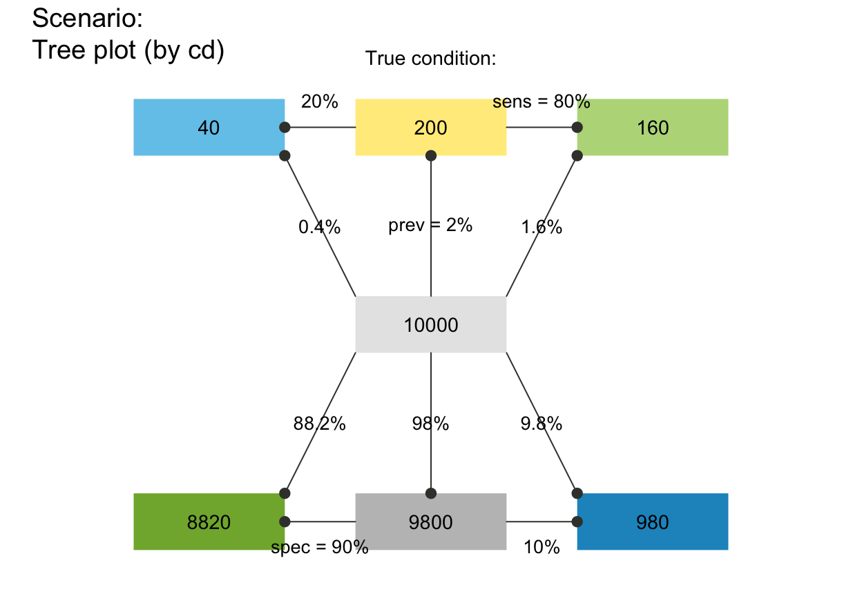
A character code specifying 1 or 2 perspective(s) that split(s) the population into 2 subsets. Specifying 1 perspective plots a frequency tree (single tree) with 3 options:
"cd": by condition only;"dc": by decision only;"ac": by accuracy only.
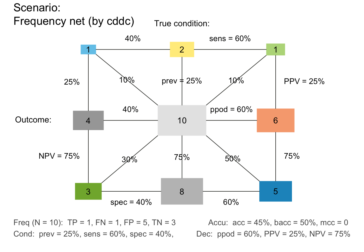
Specifying 2 perspectives plots a frequency prism (double tree) with 6 options:
"cddc": by condition (cd) and by decision (dc) (default);"cdac": by condition (cd) and by accuracy (ac);"dccd": by decision (dc) and by condition (cd);"dcac": by decision (dc) and by accuracy (ac);"accd": by accuracy (ac) and by condition (cd);"acdc": by accuracy (ac) and by decision (dc).
- area
A character code specifying the shapes of the frequency boxes, with 2 options:
"no": rectangular frequency boxes, not scaled (default);"sq": frequency boxes are squares (scaled relative to N).
- scale
Scale probabilities and corresponding area dimensions either by exact probability or by (rounded or non-rounded) frequency, with 2 options:
"p": scale main area dimensions by exact probability (default);"f": re-compute probabilities from (rounded or non-rounded) frequencies and scale main area dimensions by their frequency.
Note:
scalesetting matters for the display of probability values and for area plots with small population sizesNwhenround = TRUE.- round
Boolean option specifying whether computed frequencies are rounded to integers. Default:
round = TRUE.- sample
Boolean value that determines whether frequency values are sampled from
N, given the probability values ofprev,sens, andspec. Default:sample = FALSE.- f_lbl
Type of label for showing frequency values in 4 main areas, with 6 options:
"def": abbreviated names and frequency values;"abb": abbreviated frequency names only (as specified in code);"nam": names only (as specified inlbl_txt = txt);"num": numeric frequency values only (default);"namnum": names (as specified inlbl_txt = txt) and numeric values;"no": no frequency labels (same forf_lbl = NAorNULL).
- f_lbl_sep
Label separator for main frequencies (used for
f_lbl = "def" OR "namnum"). Usef_lbl_sep = ":\n"to add a line break between name and numeric value. Default:f_lbl_sep = NA(set to" = "or":\n"based onf_lbl).- f_lwd
Line width of areas. Default:
f_lwd = 0.- p_lwd
Line width of probability links. Default:
p_lwd = 1, but consider increasing when settingp_scale = TRUE.- p_scale
Boolean option for scaling current widths of probability links (as set by
p_lwd) by the current probability values. Default:p_scale = FALSE.- p_lbl
Type of label for showing probability links and values, with many options:
"abb": show links and abbreviated probability names;"def": show links and abbreviated probability names and values;"min": show links and minimum (prominent) probability names;"mix": show links and prominent probability names and all values (default);"nam": show links and probability names (as specified in code);"num": show links and numeric probability values;"namnum": show links with names and numeric probability values;"no": show links with no labels (same forp_lbl = NAorNULL).
- arr_c
Arrow code for symbols at ends of probability links (as a numeric value
-3 <= arr_c <= +6), with the following options:-1to-3: points at one/other/both end/s;0: no symbols;+1to+3: V-arrow at one/other/both end/s;+4to+6: T-arrow at one/other/both end/s.
Default:
arr_c = NA, but adjusted byarea.- joint_p
Boolean options for showing links to joint probabilities (i.e., diagonals from N in center to joint frequencies in 4 corners). Default:
joint_p = TRUE.- lbl_txt
Default label set for text elements. Default:
lbl_txt = txt.- main
Text label for main plot title. Default:
main = txt$scen_lbl.- sub
Text label for plot subtitle (on 2nd line). Default:
sub = "type"shows information on current plot type.- title_lbl
Deprecated text label for current plot title. Replaced by
main.- cex_lbl
Scaling factor for text labels (frequencies and headers). Default:
cex_lbl = .90.- cex_p_lbl
Scaling factor for text labels (probabilities). Default:
cex_p_lbl = cex_lbl - .05.- col_pal
Color palette. Default:
col_pal = pal.- mar_notes
Boolean option for showing margin notes. Default:
mar_notes = FALSE.- ...
Other (graphical) parameters.
Details
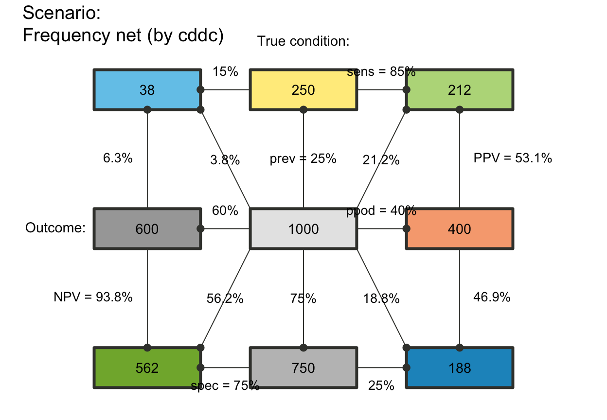
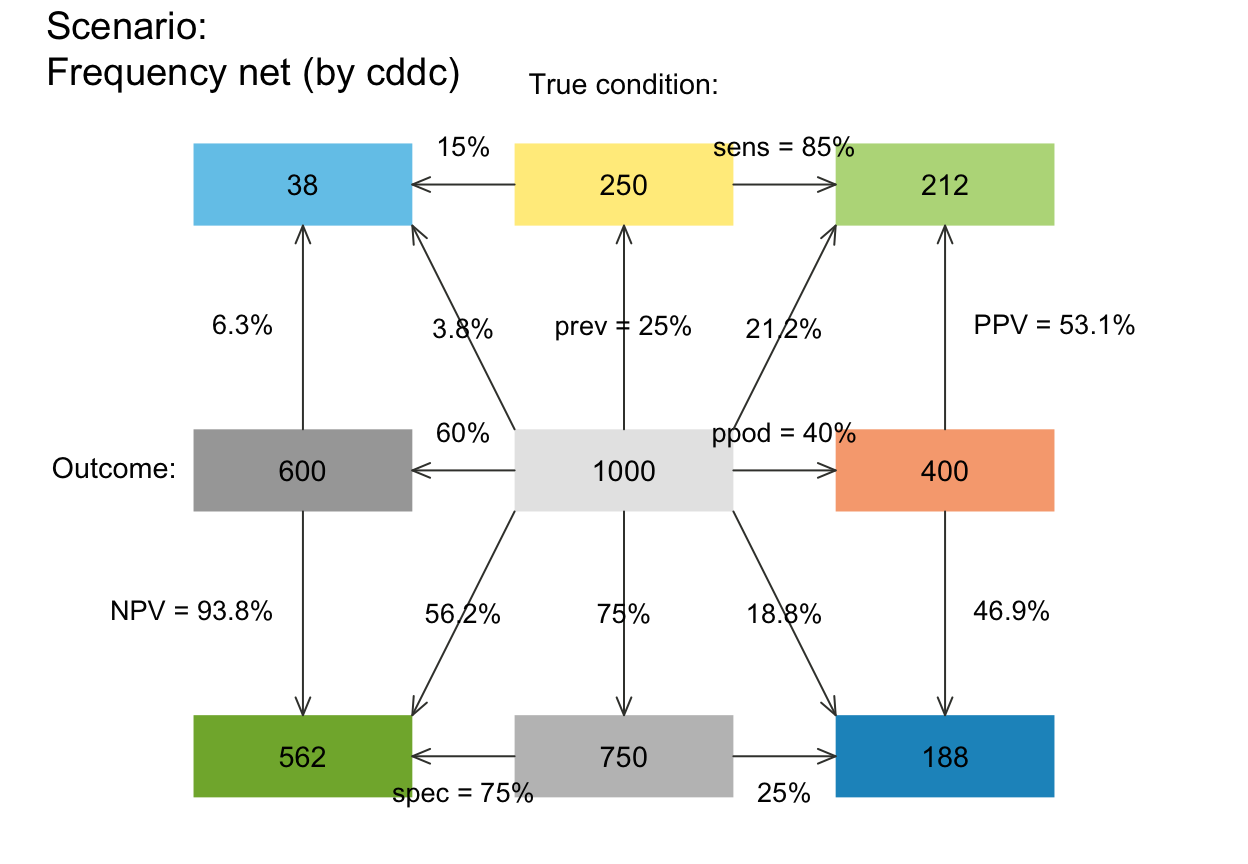
plot_fnet shows frequencies as nodes and probabilities as links
(like trees and double trees generated by plot_prism),
but combines elements from 2x2 tables (see plot_tab)
and tree diagrams.
Similar to other 2D-visualizations (e.g., ,
plot_area, plot_prism and
plot_tab), the
frequency net selects and combines two perspectives
(e.g., by = "cddc").
However, the frequency net is similar to a 2x2 table insofar as
its perspectives (shown by arranging marginal frequencies in a
vertical vs. horizontal fashion) do not suggest an order
or dependency (in contrast to trees or mosaic plots).
Additionally, the frequency net allows showing
3 kinds of (marginal, conditional, and joint) probabilities.
See the article by Binder K, Krauss S and Wiesner P (2020). A new visualization for probabilistic situations containing two binary events: The frequency net. Frontiers in Psychology, 11, 750. doi: 10.3389/fpsyg.2020.00750 for analysis and details.
See also
plot_prism for plotting prism plot (double tree);
plot_area for plotting mosaic plot (scaling area dimensions);
plot_bar for plotting frequencies as vertical bars;
plot_tab for plotting table (without scaling area dimensions);
pal contains current color settings;
txt contains current text settings.
Other visualization functions:
plot.riskyr(),
plot_area(),
plot_bar(),
plot_crisk(),
plot_curve(),
plot_icons(),
plot_mosaic(),
plot_plane(),
plot_prism(),
plot_tab(),
plot_tree()
Examples
# (1) Basics: ----
# A. Using global prob and freq values:
plot_fnet() # default frequency net, same as:
 # plot_fnet(by = "cddc", area = "no", scale = "p",
# f_lbl = "num", f_lwd = 0, cex_lbl = .90,
# p_lbl = "mix", arr_c = -2, cex_p_lbl = NA)
# B. Providing values:
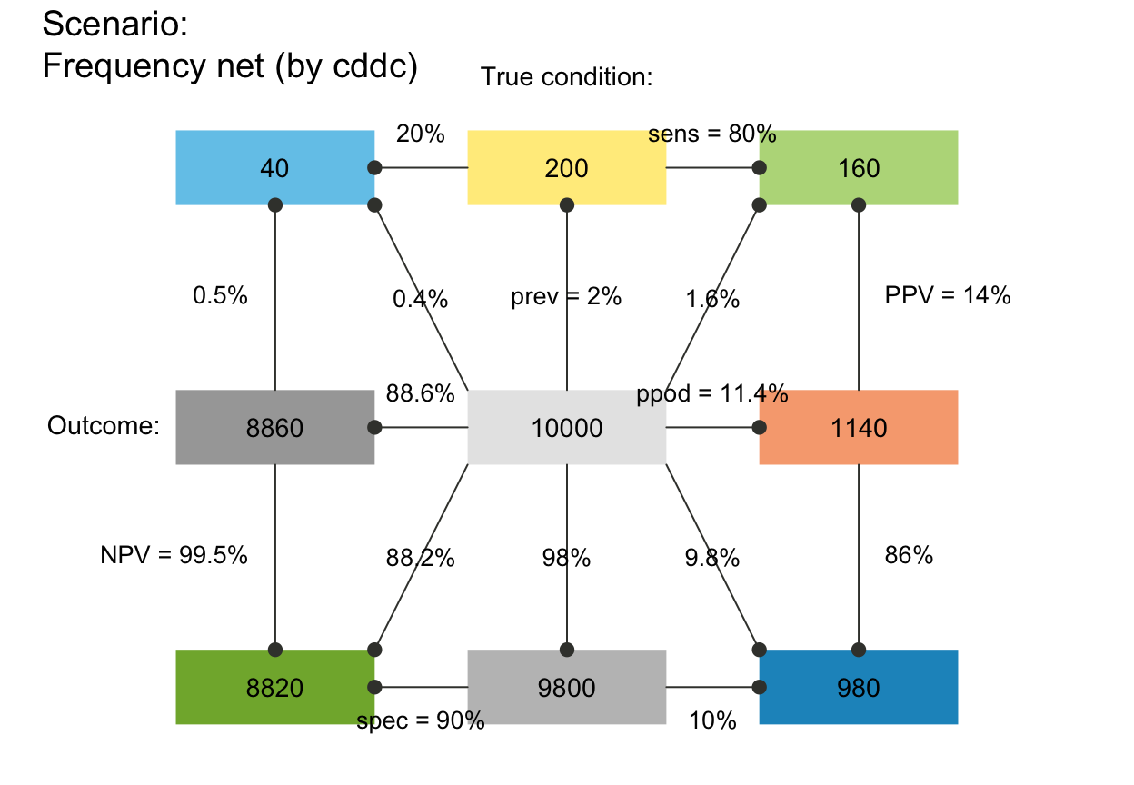
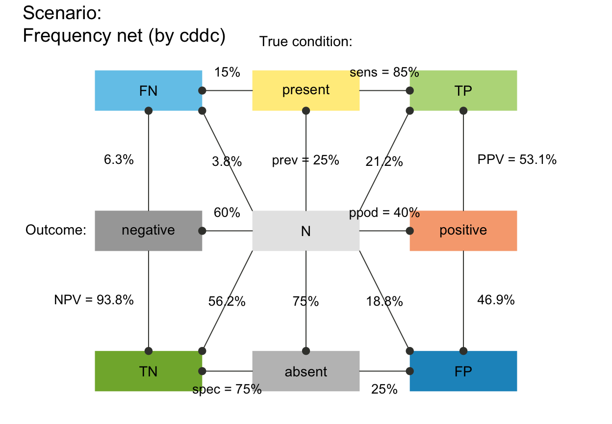
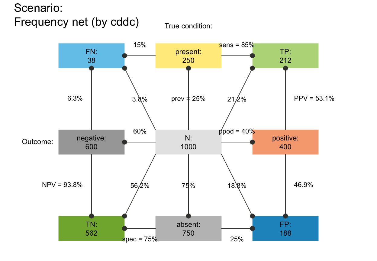
plot_fnet(N = 10000, prev = .02, sens = .8, spec = .9) # Binder et al. (2020, Fig. 3)
# plot_fnet(by = "cddc", area = "no", scale = "p",
# f_lbl = "num", f_lwd = 0, cex_lbl = .90,
# p_lbl = "mix", arr_c = -2, cex_p_lbl = NA)
# B. Providing values:
plot_fnet(N = 10000, prev = .02, sens = .8, spec = .9) # Binder et al. (2020, Fig. 3)
 # C. Rounding and sampling:
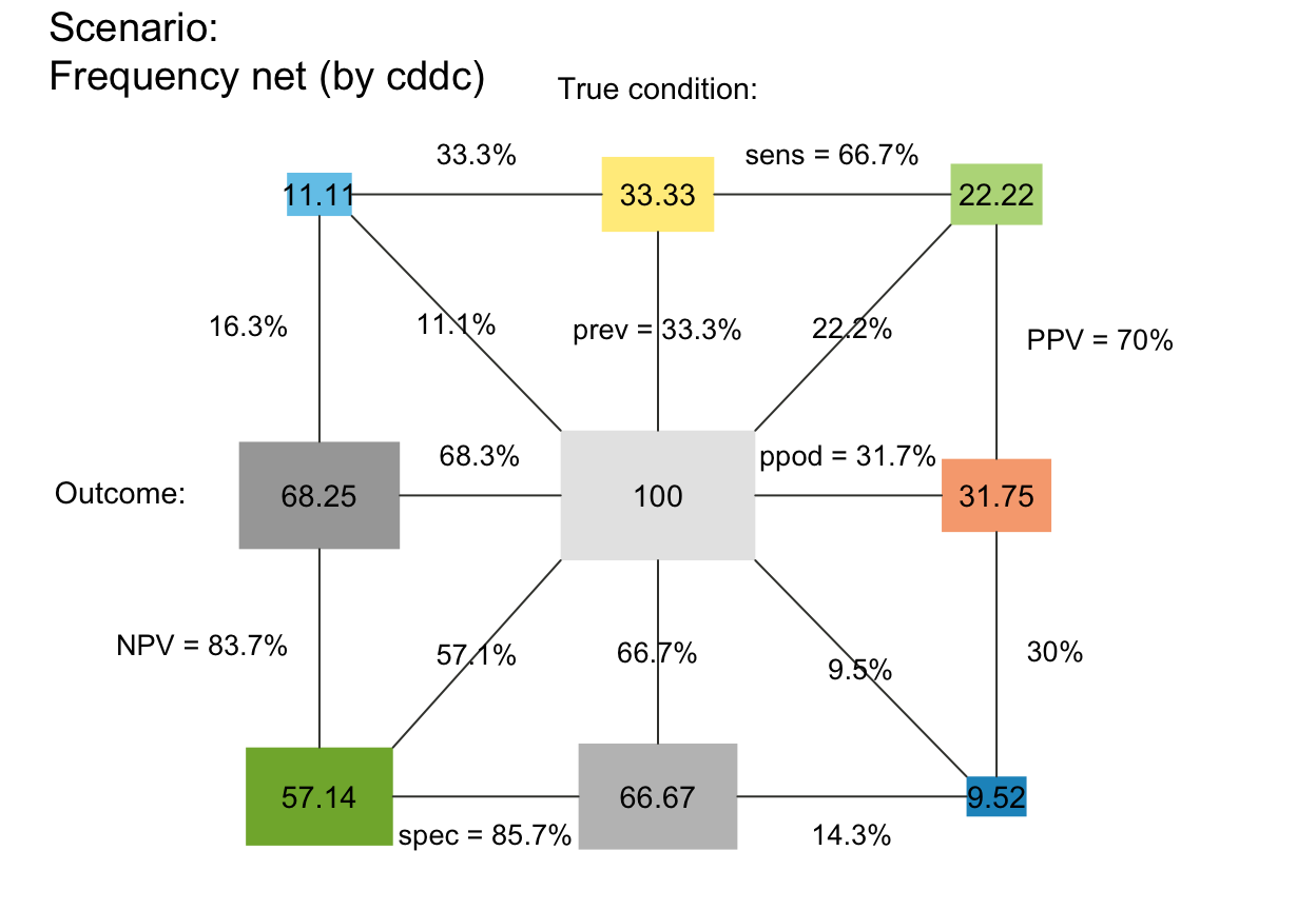
plot_fnet(N = 100, prev = 1/3, sens = 2/3, spec = 6/7, area = "sq", round = FALSE)
# C. Rounding and sampling:
plot_fnet(N = 100, prev = 1/3, sens = 2/3, spec = 6/7, area = "sq", round = FALSE)
 plot_fnet(N = 100, prev = 1/3, sens = 2/3, spec = 6/7, area = "sq", sample = TRUE, scale = "freq")
 # Variants:
plot_fnet(N = 10000, prev = .02, sens = .8, spec = .9, by = "cdac")
# Variants:
plot_fnet(N = 10000, prev = .02, sens = .8, spec = .9, by = "cdac")
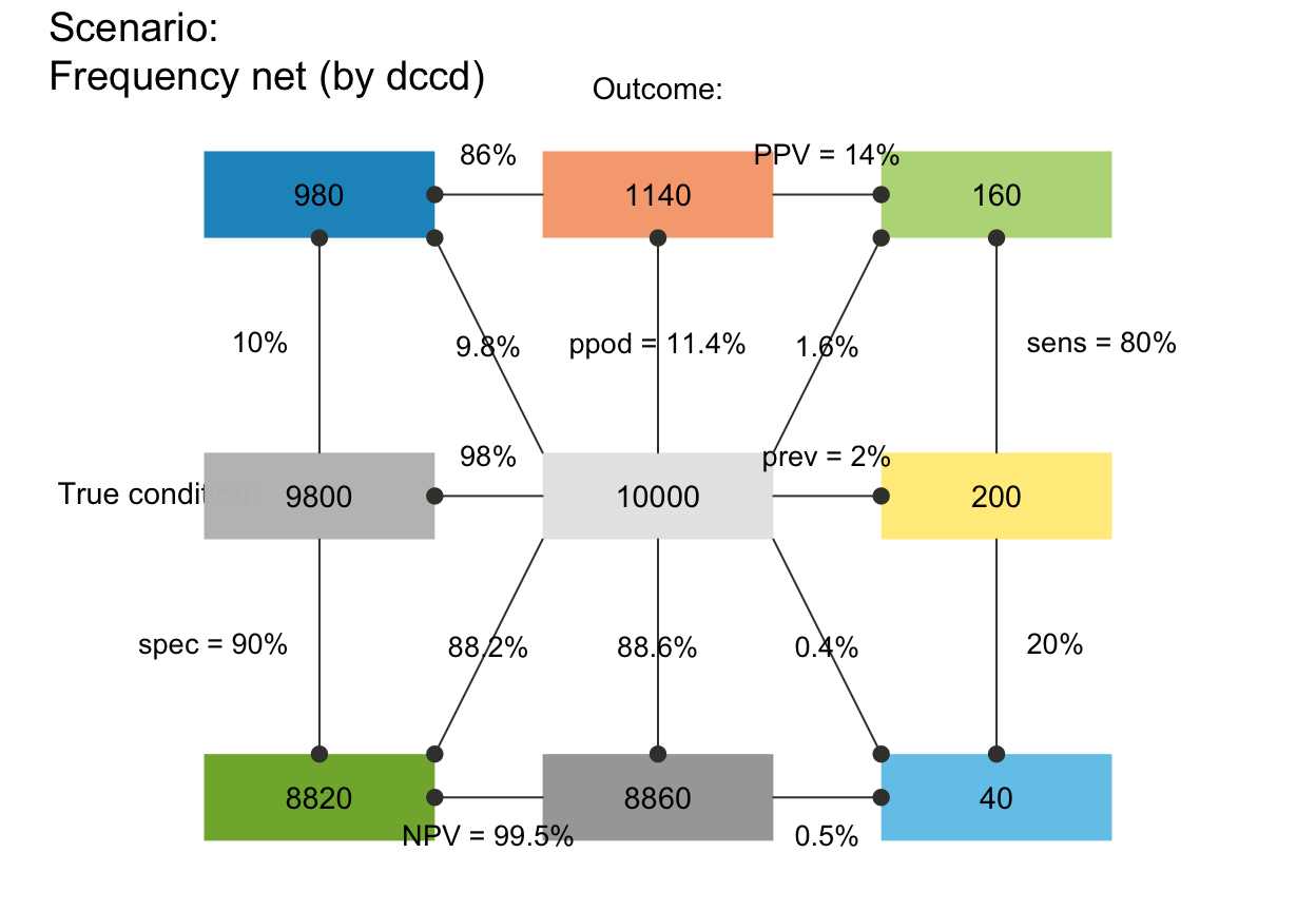
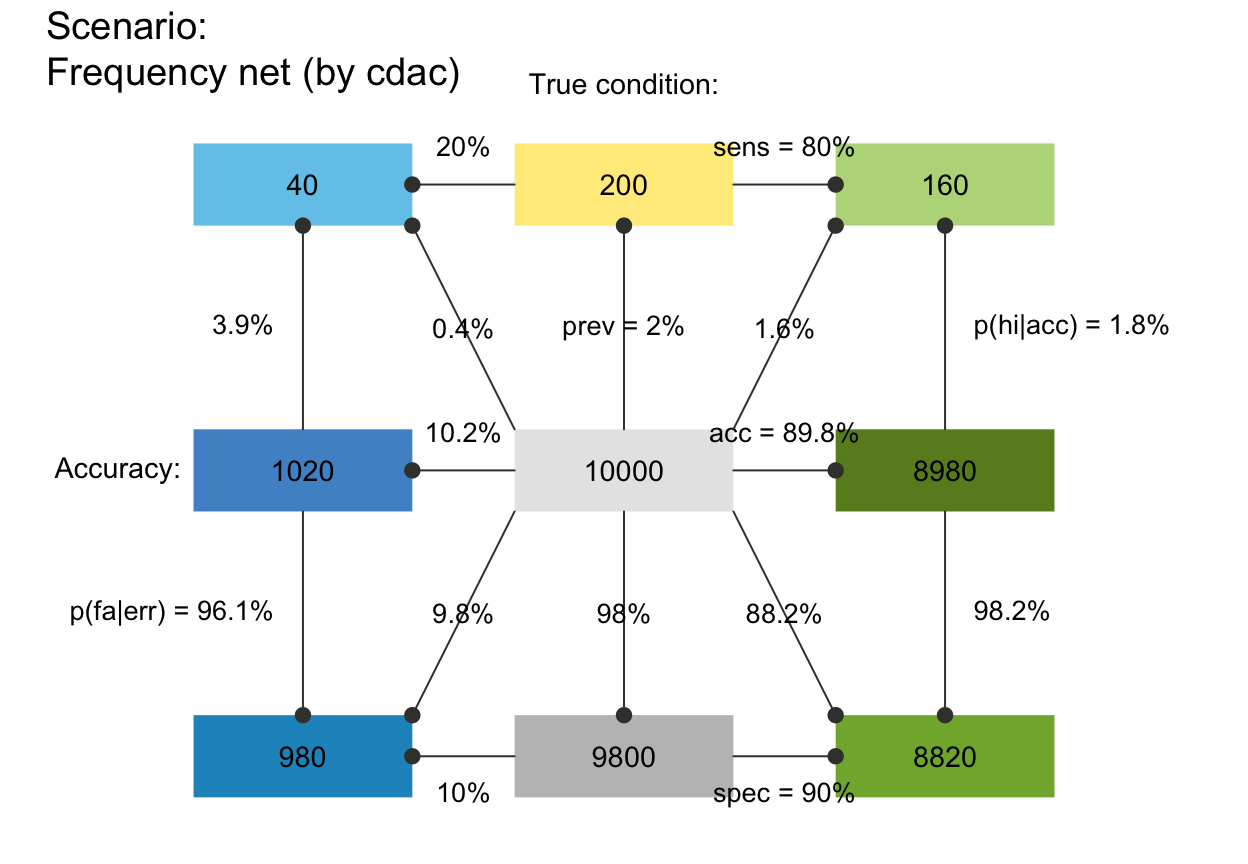 plot_fnet(N = 10000, prev = .02, sens = .8, spec = .9, by = "dccd")
 # plot_fnet(N = 10000, prev = .02, sens = .8, spec = .9, by = "dcac")
# plot_fnet(N = 10000, prev = .02, sens = .8, spec = .9, by = "accd")
# plot_fnet(N = 10000, prev = .02, sens = .8, spec = .9, by = "acdc")
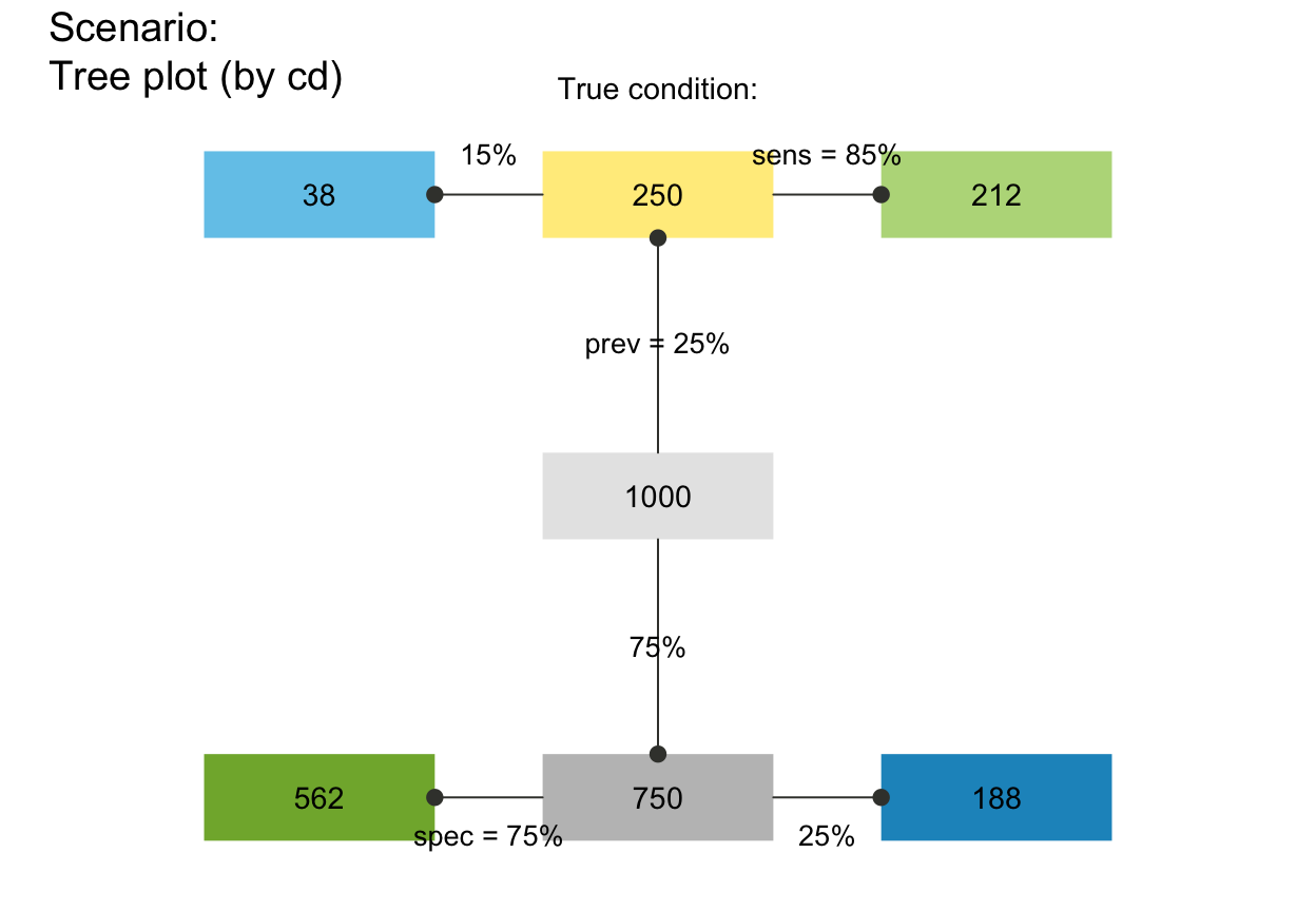
# Trees (only 1 dimension):
plot_fnet(N = 10000, prev = .02, sens = .8, spec = .9, by = "cd")
# plot_fnet(N = 10000, prev = .02, sens = .8, spec = .9, by = "dcac")
# plot_fnet(N = 10000, prev = .02, sens = .8, spec = .9, by = "accd")
# plot_fnet(N = 10000, prev = .02, sens = .8, spec = .9, by = "acdc")
# Trees (only 1 dimension):
plot_fnet(N = 10000, prev = .02, sens = .8, spec = .9, by = "cd")
 # plot_fnet(N = 10000, prev = .02, sens = .8, spec = .9, by = "dc")
# plot_fnet(N = 10000, prev = .02, sens = .8, spec = .9, by = "ac")
# Area and margin notes:
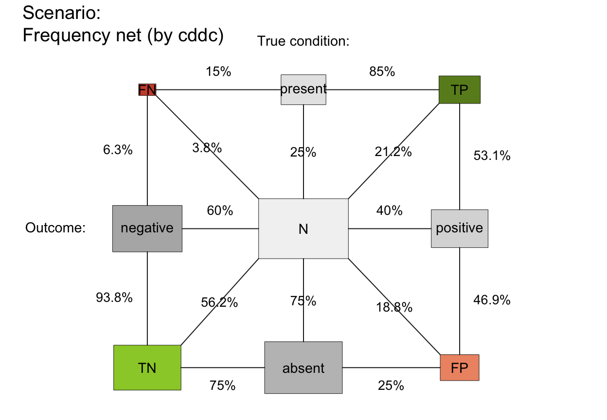
plot_fnet(N = 10, prev = 1/4, sens = 3/5, spec = 2/5, area = "sq", mar_notes = TRUE)
# plot_fnet(N = 10000, prev = .02, sens = .8, spec = .9, by = "dc")
# plot_fnet(N = 10000, prev = .02, sens = .8, spec = .9, by = "ac")
# Area and margin notes:
plot_fnet(N = 10, prev = 1/4, sens = 3/5, spec = 2/5, area = "sq", mar_notes = TRUE)
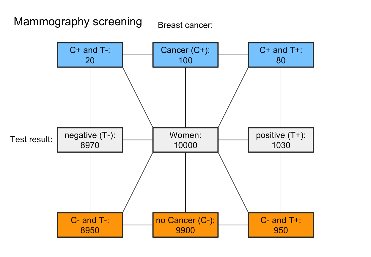
 # (2) Use case (highlight horizontal vs. vertical perspectives: ----
# Define scenario:
mammo <- riskyr(N = 10000, prev = .01, sens = .80, fart = .096,
scen_lbl = "Mammography screening", N_lbl = "Women",
cond_lbl = "Breast cancer", dec_lbl = "Test result",
cond_true_lbl = "Cancer (C+)", cond_false_lbl = "no Cancer (C-)",
dec_pos_lbl = "positive (T+)", dec_neg_lbl = "negative (T-)",
hi_lbl = "C+ and T+", mi_lbl = "C+ and T-",
fa_lbl = "C- and T+", cr_lbl = "C- and T-")
# Colors:
my_non <- "grey95"
my_red <- "orange1"
my_blu <- "skyblue1"
# A. Emphasize condition perspective (rows):
my_col_1 <- init_pal(N_col = my_non,
cond_true_col = my_blu, cond_false_col = my_red,
dec_pos_col = my_non, dec_neg_col = my_non,
hi_col = my_blu, mi_col = my_blu,
fa_col = my_red, cr_col = my_red)
plot(mammo, type = "fnet", col_pal = my_col_1,
f_lbl = "namnum", f_lwd = 2, p_lbl = "no", arr_c = 0)
# (2) Use case (highlight horizontal vs. vertical perspectives: ----
# Define scenario:
mammo <- riskyr(N = 10000, prev = .01, sens = .80, fart = .096,
scen_lbl = "Mammography screening", N_lbl = "Women",
cond_lbl = "Breast cancer", dec_lbl = "Test result",
cond_true_lbl = "Cancer (C+)", cond_false_lbl = "no Cancer (C-)",
dec_pos_lbl = "positive (T+)", dec_neg_lbl = "negative (T-)",
hi_lbl = "C+ and T+", mi_lbl = "C+ and T-",
fa_lbl = "C- and T+", cr_lbl = "C- and T-")
# Colors:
my_non <- "grey95"
my_red <- "orange1"
my_blu <- "skyblue1"
# A. Emphasize condition perspective (rows):
my_col_1 <- init_pal(N_col = my_non,
cond_true_col = my_blu, cond_false_col = my_red,
dec_pos_col = my_non, dec_neg_col = my_non,
hi_col = my_blu, mi_col = my_blu,
fa_col = my_red, cr_col = my_red)
plot(mammo, type = "fnet", col_pal = my_col_1,
f_lbl = "namnum", f_lwd = 2, p_lbl = "no", arr_c = 0)
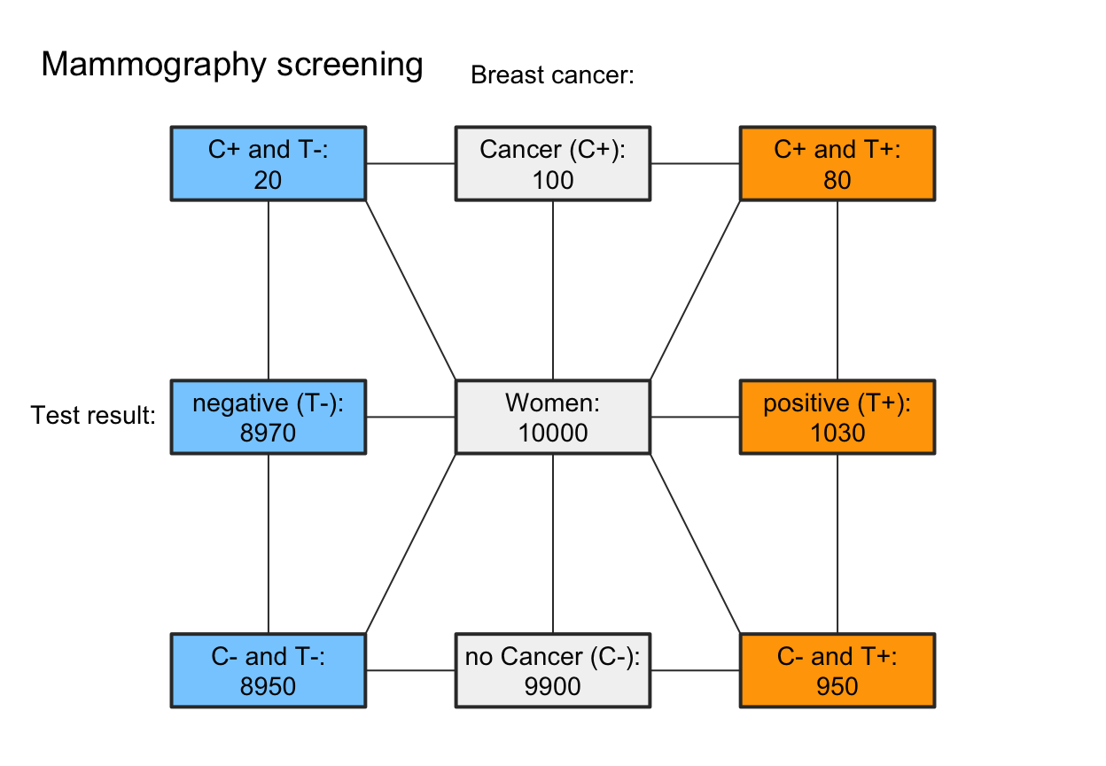
 # B. Emphasize decision perspective (columns):
my_col_2 <- init_pal(N_col = my_non,
cond_true_col = my_non, cond_false_col = my_non,
dec_pos_col = my_red, dec_neg_col = my_blu,
hi_col = my_red, mi_col = my_blu,
fa_col = my_red, cr_col = my_blu)
plot(mammo, type = "fnet", col_pal = my_col_2,
f_lbl = "namnum", f_lwd = 2, p_lbl = "no", arr_c = 0)
# B. Emphasize decision perspective (columns):
my_col_2 <- init_pal(N_col = my_non,
cond_true_col = my_non, cond_false_col = my_non,
dec_pos_col = my_red, dec_neg_col = my_blu,
hi_col = my_red, mi_col = my_blu,
fa_col = my_red, cr_col = my_blu)
plot(mammo, type = "fnet", col_pal = my_col_2,
f_lbl = "namnum", f_lwd = 2, p_lbl = "no", arr_c = 0)
 # (3) Custom color and text settings: ----
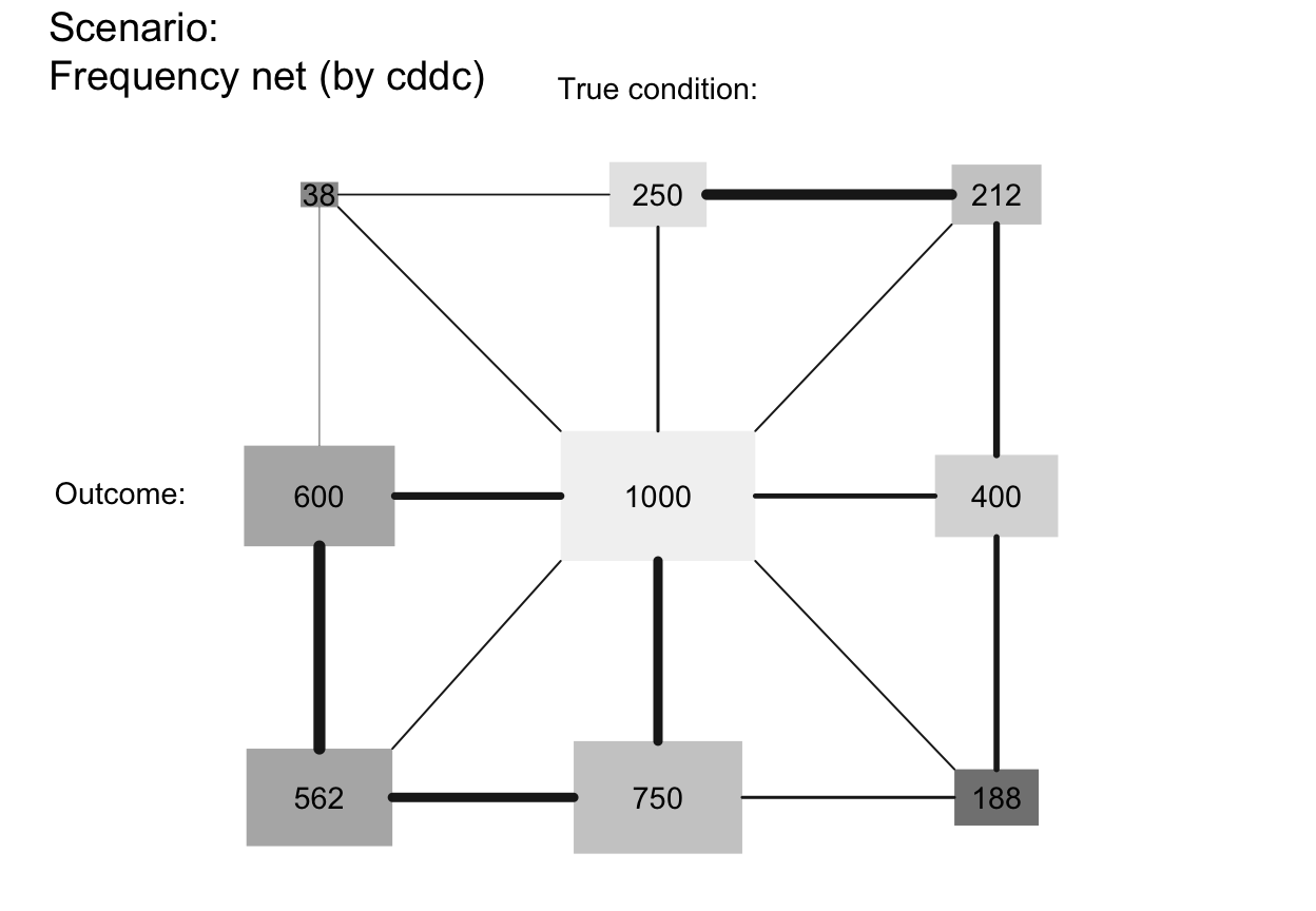
plot_fnet(col_pal = pal_bw, f_lwd = .5, p_lwd = .5, lty = 2, # custom fbox color, prob links,
font = 3, cex_p_lbl = .75) # and text labels
# (3) Custom color and text settings: ----
plot_fnet(col_pal = pal_bw, f_lwd = .5, p_lwd = .5, lty = 2, # custom fbox color, prob links,
font = 3, cex_p_lbl = .75) # and text labels
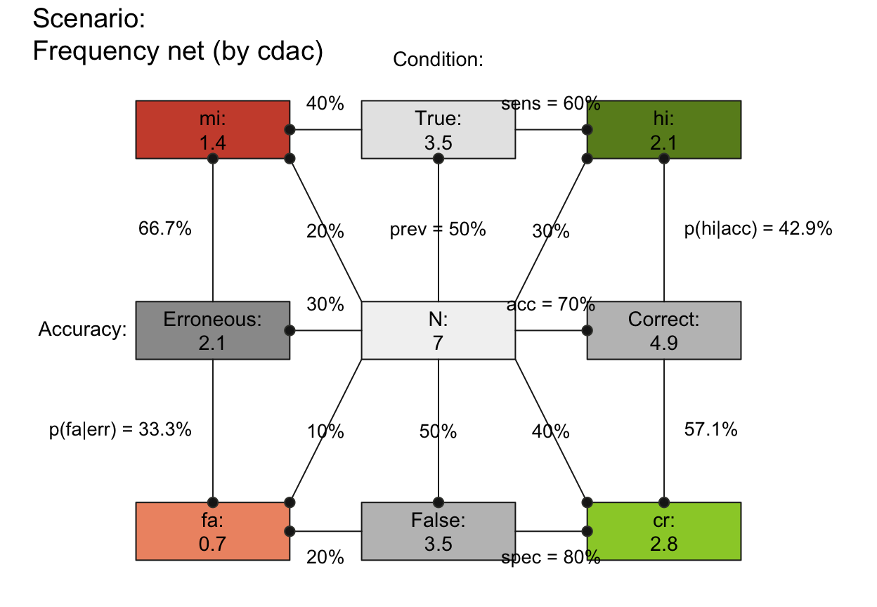
 plot_fnet(N = 7, prev = 1/2, sens = 3/5, spec = 4/5, round = FALSE,
by = "cdac", lbl_txt = txt_org, f_lbl = "namnum", f_lbl_sep = ":\n",
f_lwd = 1, col_pal = pal_rgb) # custom colors
plot_fnet(N = 7, prev = 1/2, sens = 3/5, spec = 4/5, round = FALSE,
by = "cdac", lbl_txt = txt_org, f_lbl = "namnum", f_lbl_sep = ":\n",
f_lwd = 1, col_pal = pal_rgb) # custom colors
 # plot_fnet(N = 5, prev = 1/2, sens = .8, spec = .5, scale = "p", # Note scale!
# by = "cddc", area = "hr", col_pal = pal_bw, f_lwd = 1) # custom colors
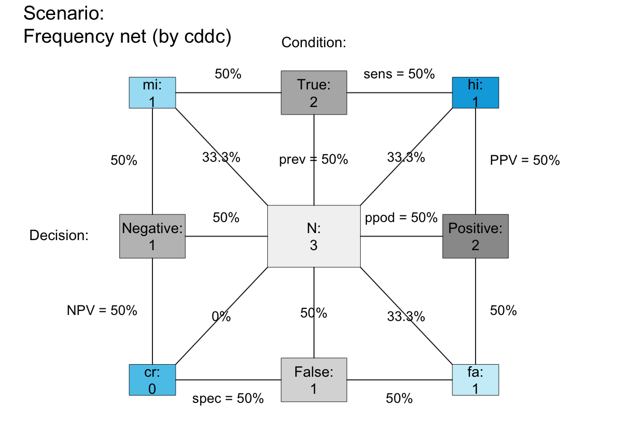
plot_fnet(N = 3, prev = .50, sens = .50, spec = .50, scale = "p", # Note scale!
area = "sq", lbl_txt = txt_org, f_lbl = "namnum", f_lbl_sep = ":\n", # custom text
col_pal = pal_kn, f_lwd = .5) # custom colors
# plot_fnet(N = 5, prev = 1/2, sens = .8, spec = .5, scale = "p", # Note scale!
# by = "cddc", area = "hr", col_pal = pal_bw, f_lwd = 1) # custom colors
plot_fnet(N = 3, prev = .50, sens = .50, spec = .50, scale = "p", # Note scale!
area = "sq", lbl_txt = txt_org, f_lbl = "namnum", f_lbl_sep = ":\n", # custom text
col_pal = pal_kn, f_lwd = .5) # custom colors
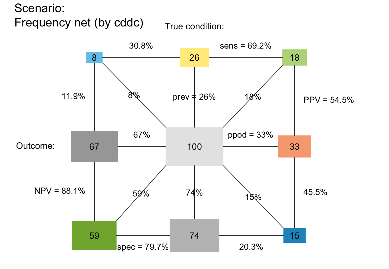
 # (4) Other options: ----
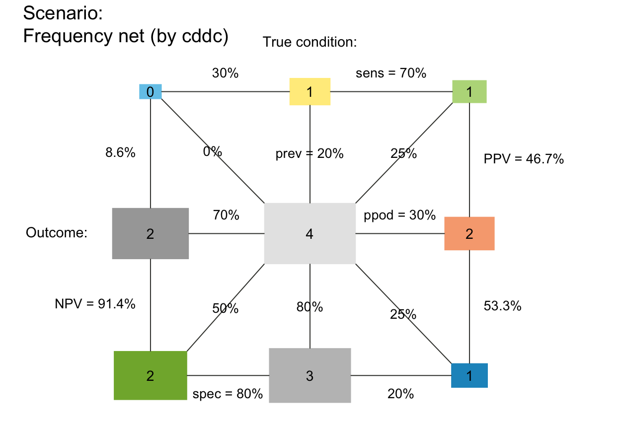
plot_fnet(N = 4, prev = .2, sens = .7, spec = .8,
area = "sq", scale = "p") # areas scaled by prob (matters for small N)
# (4) Other options: ----
plot_fnet(N = 4, prev = .2, sens = .7, spec = .8,
area = "sq", scale = "p") # areas scaled by prob (matters for small N)
 # plot_fnet(N = 4, prev = .2, sens = .7, spec = .8,
# area = "sq", scale = "f") # areas scaled by (rounded or non-rounded) freq
## Frequency boxes (f_lbl):
# plot_fnet(f_lbl = NA) # no freq labels
# plot_fnet(f_lbl = "abb") # abbreviated freq names (variable names)
plot_fnet(f_lbl = "nam") # only freq names
# plot_fnet(N = 4, prev = .2, sens = .7, spec = .8,
# area = "sq", scale = "f") # areas scaled by (rounded or non-rounded) freq
## Frequency boxes (f_lbl):
# plot_fnet(f_lbl = NA) # no freq labels
# plot_fnet(f_lbl = "abb") # abbreviated freq names (variable names)
plot_fnet(f_lbl = "nam") # only freq names
 plot_fnet(f_lbl = "num") # only numeric freq values (default)
 # plot_fnet(f_lbl = "namnum") # names and numeric freq values
plot_fnet(f_lbl = "namnum", cex_lbl = .75) # smaller freq labels
# plot_fnet(f_lbl = "namnum") # names and numeric freq values
plot_fnet(f_lbl = "namnum", cex_lbl = .75) # smaller freq labels
 # plot_fnet(f_lbl = "def") # informative default: short name and numeric value (abb = num)
# f_lwd:
# plot_fnet(f_lwd = 1) # basic lines
# plot_fnet(f_lwd = 0) # no lines (default), set to tiny_lwd = .001, lty = 0 (same if NA/NULL)
# plot_fnet(f_lwd = .5) # thinner lines
plot_fnet(f_lwd = 3) # thicker lines
# plot_fnet(f_lbl = "def") # informative default: short name and numeric value (abb = num)
# f_lwd:
# plot_fnet(f_lwd = 1) # basic lines
# plot_fnet(f_lwd = 0) # no lines (default), set to tiny_lwd = .001, lty = 0 (same if NA/NULL)
# plot_fnet(f_lwd = .5) # thinner lines
plot_fnet(f_lwd = 3) # thicker lines
 ## Probability links (p_lbl, p_lwd, p_scale):
# plot_fnet(p_lbl = NA) # no prob labels (NA/NULL/"none")
plot_fnet(p_lbl = "mix") # abbreviated names with numeric values (abb = num)
## Probability links (p_lbl, p_lwd, p_scale):
# plot_fnet(p_lbl = NA) # no prob labels (NA/NULL/"none")
plot_fnet(p_lbl = "mix") # abbreviated names with numeric values (abb = num)
 # plot_fnet(p_lbl = "min") # minimal names (of key probabilities)
# plot_fnet(p_lbl = "nam") # only prob names
plot_fnet(p_lbl = "num") # only numeric prob values
# plot_fnet(p_lbl = "min") # minimal names (of key probabilities)
# plot_fnet(p_lbl = "nam") # only prob names
plot_fnet(p_lbl = "num") # only numeric prob values
 # plot_fnet(p_lbl = "namnum") # names and numeric prob values
plot_fnet(p_lwd = 6, p_scale = TRUE)
# plot_fnet(p_lbl = "namnum") # names and numeric prob values
plot_fnet(p_lwd = 6, p_scale = TRUE)
 plot_fnet(area = "sq", f_lbl = "num", p_lbl = NA, col_pal = pal_bw, p_lwd = 6, p_scale = TRUE)
 # arr_c:
# plot_fnet(arr_c = 0) # acc_c = 0: no arrows
# plot_fnet(arr_c = -3) # arr_c = -1 to -3: points at both ends
# plot_fnet(arr_c = -2) # point at far end
plot_fnet(arr_c = +2) # crr_c = 1-3: V-shape arrows at far end
# arr_c:
# plot_fnet(arr_c = 0) # acc_c = 0: no arrows
# plot_fnet(arr_c = -3) # arr_c = -1 to -3: points at both ends
# plot_fnet(arr_c = -2) # point at far end
plot_fnet(arr_c = +2) # crr_c = 1-3: V-shape arrows at far end
 plot_fnet(by = "cd", joint_p = FALSE) # tree without joint probability links
 # plot_fnet(by = "cddc", joint_p = FALSE) # fnet ...
## Plain plot versions:
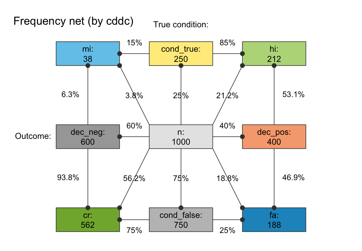
plot_fnet(area = "no", f_lbl = "def", p_lbl = "num", col_pal = pal_mod, f_lwd = 1,
main = "", mar_notes = FALSE) # remove titles and margin notes
# plot_fnet(by = "cddc", joint_p = FALSE) # fnet ...
## Plain plot versions:
plot_fnet(area = "no", f_lbl = "def", p_lbl = "num", col_pal = pal_mod, f_lwd = 1,
main = "", mar_notes = FALSE) # remove titles and margin notes
 plot_fnet(area = "no", f_lbl = "nam", p_lbl = "min", col_pal = pal_rgb)
 plot_fnet(area = "sq", f_lbl = "nam", p_lbl = "num", col_pal = pal_rgb)
 # plot_fnet(area = "sq", f_lbl = "def", f_lbl_sep = ":\n", p_lbl = NA, f_lwd = 1, col_pal = pal_kn)
## Suggested combinations:
# plot_fnet(f_lbl = "nam", p_lbl = "mix") # basic plot
plot_fnet(f_lbl = "namnum", p_lbl = "num", cex_lbl = .80, cex_p_lbl = .75)
# plot_fnet(area = "sq", f_lbl = "def", f_lbl_sep = ":\n", p_lbl = NA, f_lwd = 1, col_pal = pal_kn)
## Suggested combinations:
# plot_fnet(f_lbl = "nam", p_lbl = "mix") # basic plot
plot_fnet(f_lbl = "namnum", p_lbl = "num", cex_lbl = .80, cex_p_lbl = .75)
 # plot_fnet(area = "no", f_lbl = "def", p_lbl = "abb", # def/abb labels
# f_lwd = .8, p_lwd = .8, lty = 2, col_pal = pal_bwp) # black-&-white
# plot_fnet(area = "sq", f_lbl = "nam", p_lbl = "abb", lbl_txt = txt_TF, col_pal = pal_bw)
plot_fnet(area = "sq", f_lbl = "num", p_lbl = "num", f_lwd = 1, col_pal = pal_rgb)
# plot_fnet(area = "no", f_lbl = "def", p_lbl = "abb", # def/abb labels
# f_lwd = .8, p_lwd = .8, lty = 2, col_pal = pal_bwp) # black-&-white
# plot_fnet(area = "sq", f_lbl = "nam", p_lbl = "abb", lbl_txt = txt_TF, col_pal = pal_bw)
plot_fnet(area = "sq", f_lbl = "num", p_lbl = "num", f_lwd = 1, col_pal = pal_rgb)
 plot_fnet(area = "sq", f_lbl = "nam", p_lbl = "num", f_lwd = .5, col_pal = pal_rgb)