Data Formats
Hansjörg Neth, SPDS, uni.kn
2021 03 31
Source:vignettes/B_data_formats.Rmd
B_data_formats.RmdThe quest for certainty is the biggest obstacle to becoming risk savvy. (Gerd Gigerenzer)1
A major challenge in mastering risk literacy is coping with inevitable uncertainty. Fortunately, uncertainty in the form of risk can be expressed in terms of probabilities and thus be measured and calculated or “reckoned” with (Gigerenzer, 2002). Nevertheless, probabilistic information is often difficult to understand, even for experts in risk management and statistics. A smart and effective way to communicate probabilities is by expressing them in terms of frequencies.
Two representational formats
The problems addressed by riskyr and the scientific discussion surrounding them can be framed in terms of two representational formats: Basically, risk-related information can be expressed in terms of frequencies or in terms of probabilities (see the user guide for background information.)
riskyr reflects this basic division by
distinguishing between the same two data types and hence provides
objects that contain frequencies (specifically, a list called
freq) and objects that contain probabilities (a list called
prob). But before we explain their contents, it is
important to realize that any such separation is an abstract and
artificial one. It may make sense to distinguish frequencies from
probabilities for conceptual and educational reasons, but both in theory
and in reality both representations are intimately intertwined.2
In the following, we first consider frequencies and probabilities by themselves, before showing how both are related. As a sneak preview, the following prism plot shows both frequencies (as nodes) and probabilities (as edges connecting the nodes) from two perspectives:
library("riskyr") # load the "riskyr" package

plot_prism(prev = .01, sens = .80, spec = NA, fart = .096,  # 3 essential probabilities
           N = 1000,       # 1 frequency
           area = "no",    # same size for all boxes
           p_lbl = "abb",  # show abbreviated names of probabilities on edges
           title_lbl = "Example")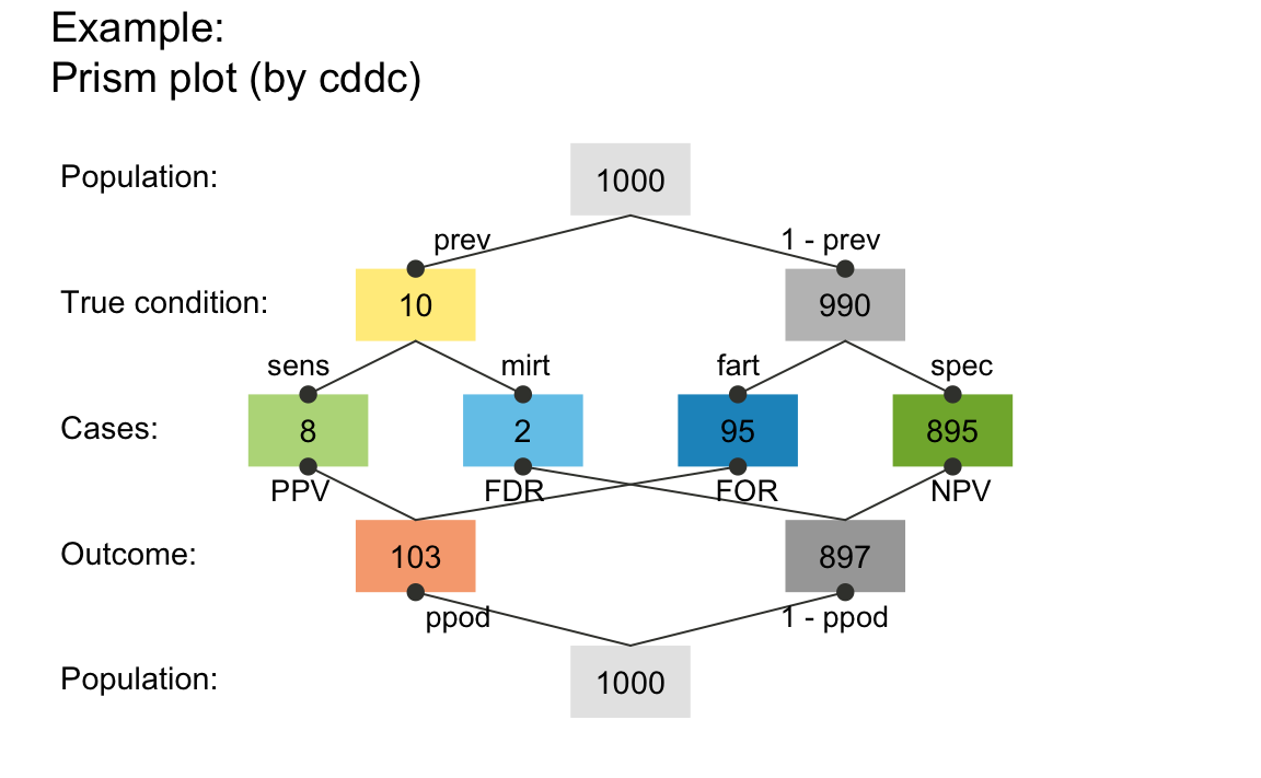
A prism plot showing frequencies as nodes and probabilities as edges linking nodes.
Frequencies
For our purposes, frequencies simply are numbers that can be counted — either 0 or positive integers.3
Definitions
The following 11 frequencies are distinguished by
riskyr and contained in freq:
| Nr. | Variable | Definition |
|---|---|---|
| 1. | N |
The number of cases (or individuals) in the population. |
| 2. | cond_true |
The number of cases for which the condition is present
(TRUE). |
| 3. | cond_false |
The number of cases for which the condition is absent
(FALSE). |
| 4. | dec_pos |
The number of cases for which the decision is positive
(TRUE). |
| 5. | dec_neg |
The number of cases for which the decision is negative
(FALSE). |
| 6. | dec_cor |
The number of cases for which the decision is correct (correspondence between decision and condition). |
| 7. | dec_err |
The number of cases for which the decision is erroneous (lack of correspondence between decision and condition). |
| 8. | hi |
The number of hits or true positives: condition present
(TRUE) & decision positive (TRUE). |
| 9. | mi |
The number of misses or false negatives: condition
present (TRUE) & decision negative
(FALSE). |
| 10. | fa |
The number of false alarms or false positives:
condition absent (FALSE) & decision positive
(TRUE). |
| 11. | cr |
The number of correct rejections or true negatives:
condition absent (FALSE) & decision negative
(FALSE). |
Perspectives: Basic vs. combined frequencies
The frequencies contained in freq can be viewed (or
parsed) from two perspectives:
Top-down: From the entire population to different parts or subgroups:
WhereasNspecifies the population size, the other 10 frequencies denote the number of individuals or cases in some subset. For instance, the frequencydec_posdenotes individuals for which the decision or diagnosis is positive. As this frequency is contained within the population, its numeric value must range from 0 toN.Bottom-up: From the 4 essential subgroups to various combinations of them:
As the 4 frequencieshi,mi,fa, andcrare not further split into subgroups, we can think of them as atomic elements or four essential frequencies. All other frequencies infreqare sums of various combinations of these four essential frequencies. This implies that the entire network of frequencies and probabilities (shown in the network diagram above) can be reconstructed from these four essential frequencies.
Relationships among frequencies
The following relationships hold among the 11 frequencies:
-
The population size
Ncan be split into several subgroups by classifying individuals by 4 different criteria:- by condition (
cd); - by decision (
dc); - by accuracy (
ac) (i.e., the correspondence of decisions to conditions); - by the combination of condition and decision (i.e., a joint category).
- by condition (
Depending on the criterion used, the following relationships hold:
Similarly, each of the subsets resulting from using the splits by
condition (cd), by
decision (dc), or by
accuracy (ac), can also be expressed as a sum of
two of the four essential frequencies. This results in three different
ways of grouping the four essential frequencies:
- by condition (
cd) (corresponding to the two columns of the confusion matrix):
- by decision (
dc) (corresponding to the two rows of the confusion matrix):
- by accuracy (
ac) (or the correspondence of decisions to conditions, corresponding to the two diagonals of the confusion matrix):
It may be tempting to refer to instances of dec_cor and
dec_err as “true decisions” and “false decisions”. However,
these terms invite conceptual confusion, as “true decisions” actually
include cond_false cases (TN or cr cases) and
“false decisions” actually include cond_true cases (FN or
mi cases).
Probabilities
The notions of probability is as elusive as ubiquitous (see Hájek, 2012, for a solid exposition of its different concepts and interpretations). For our present purposes, probabilities are simply numbers between 0 and 1. These numbers are defined to reflect particular quantities and can be expressed as percentages, as functions of and ratios between other numbers (frequencies or probabilities).
Definitions
riskyr distinguishes between 13 probabilities (see
prob for current values):
| Nr. | Variable | Name | Definition |
|---|---|---|---|
| 1. | prev |
prevalence | The probability of the condition being
TRUE. |
| 2. | sens |
sensitivity | The conditional probability of a positive
decision provided that the condition is
TRUE. |
| 3. | mirt |
miss rate | The conditional probability of a negative
decision provided that the condition is
TRUE. |
| 4. | spec |
specificity | The conditional probability of a negative
decision provided that the condition is
FALSE. |
| 5. | fart |
false alarm rate | The conditional probability of a positive
decision provided that the condition is
FALSE. |
| 6. | ppod |
proportion of positive decisions | The proportion (baseline probability or rate) of the
decision being positive (but not necessarily
TRUE). |
| 7. | PPV |
positive predictive value | The conditional probability of the condition
being TRUE provided that the decision is
positive. |
| 8. | FDR |
false detection rate | The conditional probability of the condition
being FALSE provided that the decision is
positive. |
| 9. | NPV |
negative predictive value | The conditional probability of the condition
being FALSE provided that the decision is
negative. |
| 10. | FOR |
false omission rate | The conditional probability of the condition
being TRUE provided that the decision is
negative. |
| 11. | acc |
accuracy | The probability of a correct decision (i.e., correspondence of decisions to conditions). |
| 12. | p_acc_hi |
– | The conditional probability of the condition
being TRUE provided that a decision or prediction is
accurate. |
| 13. | p_err_fa |
– | The conditional probability of the condition
being FALSE provided that a decision or prediction is
inaccurate or erroneous. |
Note that the prism diagram (plot_prism) shows a total
of 18 probabilities: 3 perspectives (by = "cd",
by = "dc", and by = "ac") and 6 edges denoting
the (marginal and conditional) probabilities for each perspective.
However, we currently do not explicitly identify all possible
probabilities.4
Non-conditional vs. conditional probabilities
Note that a typical riskyr scenario contains several marginal or non-conditional probabilities:
- The prevalence
prev(1.) only depends on features of the condition. - The proportion of positive decisions
ppod(or bias) (6.) only depends on features of the decision. - The accuracy
acc(11.) depends onprevandppod, but unconditionally dissects a population into two groups (dec_corvs.dec_err).
The other probabilities are conditional probabilities based on three perspectives:
- by condition: conditional probabilities (2. to 5.) depend
on the condition’s
prevand features of the decision.
- by decision: conditional probabilities (7. to 10.) depend
on the decision’s
ppodand features of the condition.
- by accuracy: conditional probabilities based on
accuracy
accare currently computed, but – in the absence of a commonly accepted term — namedp_acc_hiandp_err_fa(12. and 13.).
Relationships among probabilities
The following relationships hold among the conditional probabilities:
- The sensitivity
sensand miss ratemirtare complements:
- The specificity spec and
false alarm rate fart are complements:
- The positive predictive
value PPV and false detection rate FDR are
complements:
- The negative predictive
value NPV and false omission rate FOR are
complements:
It is possible to adapt Bayes’ formula to define PPV
and NPV in terms of prev, sens,
and spec:
$$ \texttt{PPV} = \frac{\texttt{prev} \cdot \texttt{sens}}{\texttt{prev} \cdot \texttt{sens} + (1 - \texttt{prev}) \cdot (1 - \texttt{sens})}\\ \\ \\ \texttt{NPV} = \frac{(1 - \texttt{prev}) \cdot \texttt{spec}}{\texttt{prev} \cdot (1 - \texttt{sens}) + (1 - \texttt{prev}) \cdot \texttt{spec}} $$
Although this is how the functions comp_PPV and
comp_NPV compute the desired conditional probability, it is
difficult to remember and think in these terms. Instead, we recommend
thinking about and defining all conditional probabilities in terms of
frequencies and relations between frequencies (see Neth et al., 2021
for details).
Probabilities as ratios between frequencies
The easiest way to think about, define, and compute the probabilities
(contained in prob) is in terms of frequencies (contained
in freq):
| Nr. | Variable | Name | Definition | as Frequencies |
|---|---|---|---|---|
| 1. | prev |
prevalence | The probability of the condition being
TRUE. |
prev =
cond_true/N
|
| 2. | sens |
sensitivity | The conditional probability of a positive
decision provided that the condition is
TRUE. |
sens =
hi/cond_true
|
| 3. | mirt |
miss rate | The conditional probability of a negative
decision provided that the condition is
TRUE. |
mirt =
mi/cond_true
|
| 4. | spec |
specificity | The conditional probability of a negative
decision provided that the condition is
FALSE. |
spec =
cr/cond_false
|
| 5. | fart |
false alarm rate | The conditional probability of a positive
decision provided that the condition is
FALSE. |
fart =
fa/cond_false
|
| 6. | ppod |
proportion of positive decisions | The proportion (baseline probability or rate) of the
decision being positive (but not necessarily
TRUE). |
ppod =
dec_pos/N
|
| 7. | PPV |
positive predictive value | The conditional probability of the condition
being TRUE provided that the decision is
positive. |
PPV =
hi/dec_pos
|
| 8. | FDR |
false detection rate | The conditional probability of the condition
being FALSE provided that the decision is
positive. |
FDR =
fa/dec_pos
|
| 9. | NPV |
negative predictive value | The conditional probability of the condition
being FALSE provided that the decision is
negative. |
NPV =
cr/dec_neg
|
| 10. | FOR |
false omission rate | The conditional probability of the condition
being TRUE provided that the decision is
negative. |
FOR =
mi/dec_neg
|
| 11. | acc |
accuracy | The probability of a correct decision (i.e., correspondence of decisions to conditions). |
acc =
dec_cor/N
|
| 12. | p_acc_hi |
– | The conditional probability of the condition
being TRUE provided that a decision or prediction is
accurate. |
p_acc_hi =
hi/dec_cor
|
| 13. | p_err_fa |
– | The conditional probability of the condition
being FALSE provided that a decision or prediction is
inaccurate or erroneous. |
p_err_fa =
fa/dec_err
|
Note that the ratios between frequencies are straightforward consequences of the probabilities’ definitions:
-
The unconditional probabilities (1., 6. and 11.) are proportions of the entire population:
-
prev=cond_true/N -
ppod=dec_pos/N -
acc=dec_cor/N
-
The conditional probabilities (2.–5., 7.–10., and 11.–12.) can be computed as a proportion of the reference group on which they are conditional. More specifically, if we schematically read each definition as “The conditional probability of provided that ”, then the ratio of the corresponding frequencies is
X & Y/Y. More explicitly,
- the ratio’s numerator is the frequency of the joint occurrence
(i.e., both
X & Y) being the case; - the ratio’s denominator is the frequency of the condition
(
Y) being the case.
When computing probabilities from rounded frequencies, their numeric
values may deviate from the true underlying probabilities, particularly
for small population sizes N. (Use the scale
argument of many riskyr plotting functions to control
whether probabilities are based on frequencies.)
Practice
An example
The following prism (or network) diagram is based on the following inputs:
- a condition’s prevalence of 50% (
prev = .50); - a decision’s sensitivity of 80% (
sens = .80); - a decision’s specificity of 60% (
spec = .60); - a population size of 10 individuals (
N = 10);
and illustrates the relationship between frequencies and probabilities:
plot_prism(prev = .50, sens = .80, spec = .60,  # 3 essential probabilities
           N = 10,         # population frequency
           scale = "f",    # scale by frequency, rather than probability ("p")
           area = "sq",    # boxes as squares, with sizes scaled by current scale
           p_lbl = "num",  # show numeric probability values on edges
           title_lbl = "Probabilities as ratios between frequencies")
#> Argument 'title_lbl' is deprecated. Please use 'main' instead.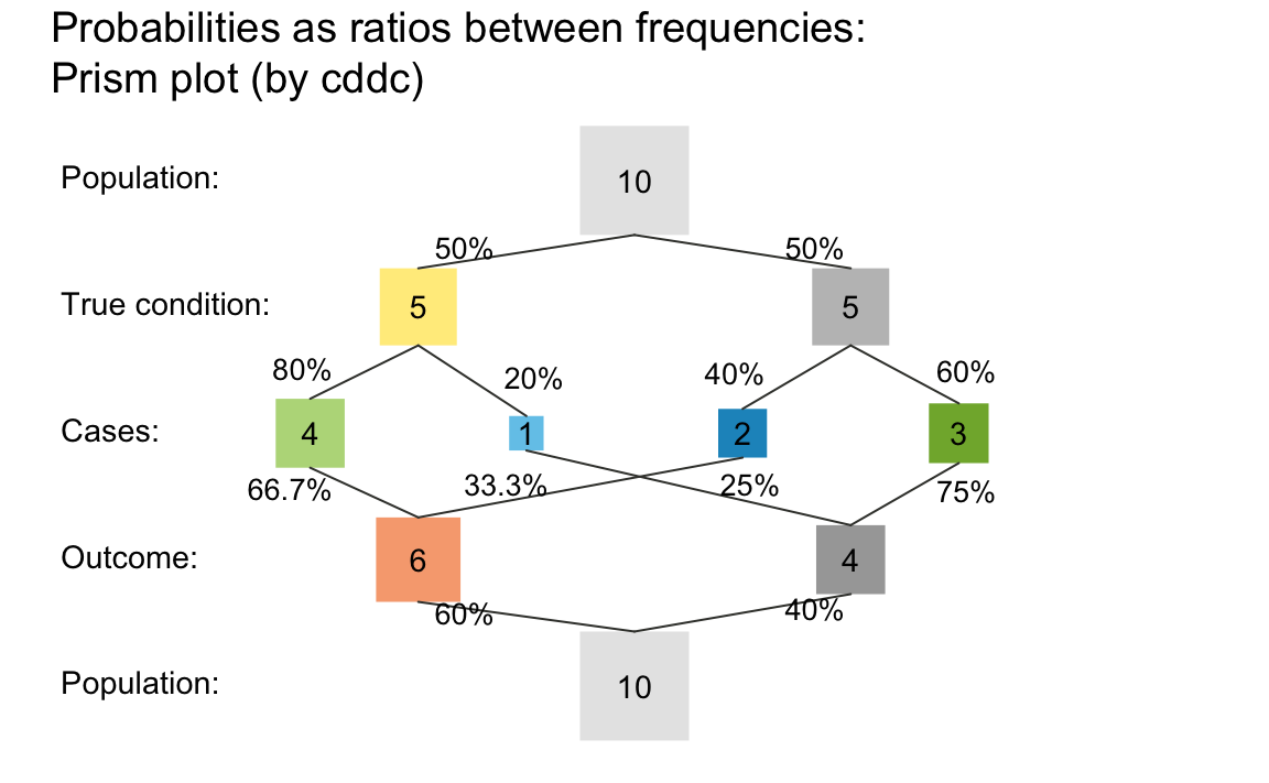
A prism plot showing how probabilities can be computed as ratios between frequencies.
Your tasks
Verify that the probabilities (shown as numeric values on the edges) match the ratios of the corresponding frequencies (shown in the boxes). What are the names of these probabilities?
What is the frequency of
dec_coranddec_errcases? Where do these cases appear in the diagram?The parameter values in the example do not require any rounding of frequencies. Change them (e.g., to
N = 5) and explore what happens when alternating betweenscale = "f"andscale = "p".
References
Gigerenzer, G. (2002). Reckoning with risk: Learning to live with uncertainty. London, UK: Penguin.
Gigerenzer, G. (2014). Risk savvy: How to make good decisions. New York, NY: Penguin.
Gigerenzer, G., & Hoffrage, U. (1999). Overcoming difficulties in Bayesian reasoning: A reply to Lewis and Keren (1999) and Mellers and McGraw (1999). Psychological Review, 106, 425–430.
Hájek, A (2012) Interpretations of Probability. In Edward N. Zalta (Ed.), The Stanford Encyclopedia of Philosophy. URL: https://plato.stanford.edu/entries/probability-interpret/ 2012 Archive
Hoffrage, U., Gigerenzer, G., Krauss, S., & Martignon, L. (2002). Representation facilitates reasoning: What natural frequencies are and what they are not. Cognition, 84, 343–352.
Neth, H., Gradwohl, N., Streeb, D., Keim, D.A., & Gaissmaier, W. (2021). Perspectives on the 2x2 matrix: Solving semantically distinct problems based on a shared structure of binary contingencies. Frontiers in Psychology: Cognition, 11, 567817. doi: 10.3389/fpsyg.2020.567817 (Available online)
Trevethan, R. (2017). Sensitivity, specificity, and predictive values: Foundations, pliabilities, and pitfalls in research and practice. Frontiers in Public Health, 5, 307. (Available online)
Resources
The following resources and versions are currently available:
| Type: | Version: | URL: |
|---|---|---|
| A. riskyr (R package): | Release version | https://CRAN.R-project.org/package=riskyr |
| Development version | https://github.com/hneth/riskyr/ | |
| B. riskyrApp (R Shiny code): | Online version | https://riskyr.org/ |
| Development version | https://github.com/hneth/riskyrApp/ | |
| C. Online documentation: | Release version | https://hneth.github.io/riskyr/ |
| Development version | https://hneth.github.io/riskyr/dev/ |
Contact
![]()
We appreciate your feedback, comments, or questions.
Please report any riskyr-related issues at https://github.com/hneth/riskyr/issues/.
Contact us at contact.riskyr@gmail.com with any comments, questions, or suggestions.
All riskyr vignettes

| Nr. | Vignette | Content |
|---|---|---|
| A. | User guide | Motivation and general instructions |
| B. | Data formats | Data formats: Frequencies and probabilities |
| C. | Confusion matrix | Confusion matrix and accuracy metrics |
| D. | Functional perspectives | Adopting functional perspectives |
| E. | Quick start primer | Quick start primer |