Confusion Matrix and Metrics

Hansjörg Neth, SPDS, uni.kn

2021 03 31

Behold the aptly named “confusion matrix”:

	Condition
Decision	present (TRUE):	absent (FALSE):	Sum:	(b) by decision:
positive (TRUE):	hi	fa	dec_pos	PPV = hi/dec_pos
negative (FALSE):	mi	cr	dec_neg	NPV = cr/dec_neg
Sum:	cond_true	cond_false	N	prev = cond_true/N
(a) by condition	sens = hi/cond_true	spec = cr/cond_false	ppod = dec_pos/N	acc = dec_cor/N = (hi+cr)/N

Most people, including medical experts and social scientists, struggle to understand the implications of this matrix. This is no surprise when considering explanations like the corresponding article on Wikipedia, which squeezes more than a dozen metrics out of four essential frequencies (hi, mi, fa, and cr). While each particular metric is quite simple, their abundance and inter-dependence can be overwhelming.

Fortunately, the key representational structure can also be understood as a 2x2 matrix (aka. 2-by-2 contingency table), which is actually quite simple, and rather straightforward in its implications. In the following, we identify the most important aspects and some key measures that a risk-literate person should know (see Neth et al., 2021, for a more detailed account).

Basics

Condensed to its core, the 2x2 matrix cross-tabulates (or “confuses”) two binary dimensions and classifies each individual case into one of four possible categories that result from combining the two binary variables (e.g., the condition and decision of each case) with each other. This sounds more complicated than it is:

	Condition
Decision	present (TRUE):	absent (FALSE):
positive (TRUE):	hi	fa
negative (FALSE):	mi	cr

Fortunately, this table is not so confusing any more: It shows four frequency counts (or “joint” frequencies) that result from cross-tabulating two binary dimensions. And, perhaps surprisingly, all other metrics of interest in various contexts and domains follow from this simple core in a straightforward way. In the following, we illustrate how the other metrics can be constructed from the four essential frequencies.

Adopting two perspectives on a population

Essentially, the confusion matrix views a population of N individuals in different ways by adopting different perspectives. “Adopting a perspective” means that we can distinguish between individuals on the basis of some criterion. The two primary criteria used here are:

(a) each individual’s condition, which can either be present (TRUE) or absent (FALSE), and
(b) each individual’s decision, which can either be positive (TRUE) or negative (FALSE).

Numerically, the adoption of each of these two perspectives splits the population into two subgroups.¹ Applying two different splits of a population into two subgroups results in $2 \times 2 = 4$ cases, which form the core of the confusion matrix:

1. hi represents hits (or true positives): condition present (TRUE) & decision positive (TRUE).
2. mi represents misses (or false negatives): condition present (TRUE) & decision negative (FALSE).
3. fa represents false alarms (or false positives): condition absent (FALSE) & decision positive (TRUE).
4. cr represents correct rejections (or true negatives): condition absent (FALSE) & decision negative (FALSE).

Importantly, all frequencies required to understand and compute various metrics are combinations of these four frequencies — which is why we refer to them as the four essential frequencies (see the vignette on Data formats). For instance, adding up the columns and rows of the matrix yields the frequencies of the two subgroups that result from adopting our two perspectives on the population N (or splitting N into subgroups by applying two binary criteria):

(a) by condition (cd) (corresponding to the two columns of the confusion matrix):

$$\begin{aligned} \texttt{N} \ &= \ \texttt{cond_true} & +\ \ \ \ \ &\texttt{cond_false} & \textrm{(a)} \\ \ &= \ (\texttt{hi} + \texttt{mi}) & +\ \ \ \ \ &(\texttt{fa} + \texttt{cr}) \\ \end{aligned}$$

(b) by decision (dc) (corresponding to the two rows of the confusion matrix):

$$\begin{aligned} \texttt{N} \ &= \ \texttt{dec_pos} & +\ \ \ \ \ &\texttt{dec_neg} & \ \ \ \ \textrm{(b)} \\ \ &= \ (\texttt{hi} + \texttt{fa}) & +\ \ \ \ \ &(\texttt{mi} + \texttt{cr}) \\ \end{aligned}$$

To reflect these two perspectives in the confusion matrix, we only need to add the sums of columns (i.e., by condition) and rows (by decision):

	Condition
Decision	present (TRUE):	absent (FALSE):	Sum:
positive (TRUE):	hi	fa	dec_pos
negative (FALSE):	mi	cr	dec_neg
Sum:	cond_true	cond_false	N

An third perspective is provided by considering the diagonals of the 2x2 matrix. In many semantic domains, the diagonals denote the accuracy of the classification, or the correspondence between dimensions (see below).

Example

To view a 2x2 matrix (or confusion table) in riskyr, we can use the plot_tab() function (i.e., plot an existing scenario as type = "tab"):

## (1) Plot table from basic input parameters: ----- 
plot_tab(prev = .05, sens = .75, spec = .66, N = 1000,
         p_lbl = "def") # show condition probabilies (by default)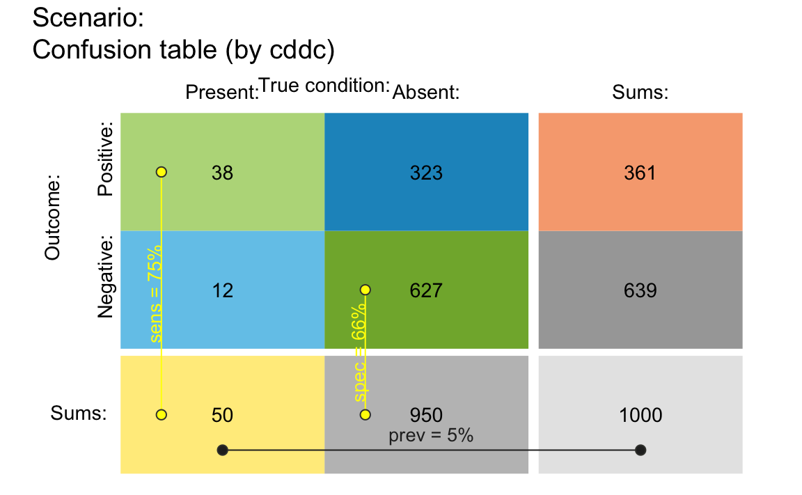

Example of a 2x2 confusion table in riskyr.

Accuracy as a third perspective

A third way of grouping the four essential frequencies results from asking the question: Which of the four essential frequencies are correct decisions and which are erroneous decisions? Crucially, this question about decision accuracy can neither be answered by only considering each individual’s condition (i.e., the columns of the matrix), nor can it be answered by only considering each individual’s decision (i.e., the rows of the matrix). Instead, answering the question about accuracy requires that the other dimensions have been determined and then considering the correspondence between condition and decision. Checking the correspondence between rows and columns for the four essential frequencies yields an important insight: The confusion matrix contains two types of correct decisions and two types of errors:

• A decision is correct, when it corresponds to the condition. This is the case for two cells in (or the “" diagonal of) the confusion matrix:

  • hi: condition present (TRUE) & decision positive (TRUE)
  • cr: condition absent (FALSE) & decision negative (FALSE)

• A decision is incorrect or erroneous, when it does not correspond to the condition. This also is the case for two cells in (or the “/” diagonal of) the confusion matrix:

  • mi: condition present (TRUE) & decision negative (FALSE)
  • fa: condition absent (FALSE) & decision positive (TRUE)

Splitting all N individuals into two subgroups of those with correct vs. those with erroneous decisions yields a third perspective on the population:

(c) by accuracy (ac) or the correspondence between decisions and conditions (corresponding to the two diagonals of the confusion matrix):

$$\begin{aligned} \texttt{N} \ &= \ \texttt{dec_cor} & +\ \ \ \ \ &\texttt{dec_err} & \ \ \textrm{(c)} \\ \ &= \ (\texttt{hi} + \texttt{cr}) & +\ \ \ \ \ &(\texttt{mi} + \texttt{fa}) \\ \end{aligned}$$

Example

Re-arranging the cells of the 2x2 matrix allows illustrating accuracy as a third perspective (e.g., by specifying the perspective by = "cdac"):

plot_tab(prev = .05, sens = .75, spec = .66, N = 1000,
         by = "cdac", p_split = "h", 
         p_lbl = "def", title_lbl = "Scenario 2")
#> Argument 'title_lbl' is deprecated. Please use 'main' instead.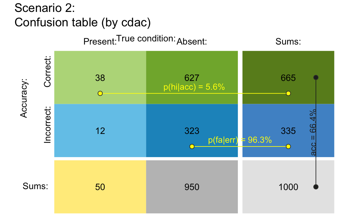

Arranging a 2x2 confusion table by condition and by accuracy.

Avoiding common sources of confusion

It may be instructive to point out two possible sources of confusion, so that they can be deliberately avoided:

1. Beware of alternative terms for mi and cr:

   • Misses mi are often called “false negatives” (FN), but are nevertheless cases for which the condition is TRUE (i.e., in the cond_true column of the confusion table).

   • Correct rejections cr are often called “true negatives” (TN), but are nevertheless cases for which the condition is FALSE (i.e., in the cond_false column of the confusion table).

Thus, the terms “true” and “false” are sometimes ambiguous by switching their referents. When used to denote the four essential frequencies (e.g., describing mi as “false negatives” and cr as “true negatives”) the terms refer to the correspondence of a decision to the condition, rather than to their condition. To avoid this source of confusion, we prefer the terms mi and cr over “false negatives” (FN) and “true negatives” (TN), respectively, but offer both options as pre-defined lists of text labels (see txt_org and txt_TF).

2. Beware of alternative terms for dec_cor and dec_err:
   Similarly, it may be tempting to refer to instances of dec_cor and dec_err as “true decisions” and “false decisions”. However, this would also invite conceptual confusion, as “true decisions” would include cond_false cases (cr or TN cases) and “false decisions” would include cond_true cases (mi or FN cases). Again, we prefer the less ambiguous terms “correct decisions” vs. “erroneous decisions”.

Accuracy metrics

The perspective of accuracy raises an important question: How good is some decision process (e.g., a clinical judgment or some diagnostic test) in capturing the true state of the condition? Different accuracy metrics provide different answers to this question, but share a common goal — measuring decision performance by capturing the correspondence of decisions to conditions in some quantitative fashion.²

While all accuracy metrics quantify the relationship between correct and erroneous decisions, different metrics emphasize different aspects or serve different purposes. We distinguish between specific and general metrics.

A. Specific metrics: Conditional probabilities

The goal of a specific accuracy metric is to quantify some particular aspect of decision performance. For instance, how accurate is our decision or diagnostic test in correctly detecting cond_true cases? How accurate is it in detecting cond_false cases?

As we are dealing with two types of correct decisions (hi and cr) and two perspectives (by columns vs. by rows), we can provide 4 answers to these questions. To obtain a numeric quantity, we divide the frequency of correct cases (either hi or cr) by

(a) column sums (cond_true vs. cond_false): This yields the decision’s sensitivity (sens) and specificity (spec):

$$\begin{aligned} \texttt{sens} \ &= \frac{\texttt{hi}}{\texttt{cond_true}} & \ \ \textrm{(a1)} \\ \ \\ \texttt{spec} \ &= \frac{\texttt{cr}}{\texttt{cond_false}} & \ \ \textrm{(a2)} \\ \end{aligned}$$

(b) row sums (dec_pos vs. dec_neg): This yields the decision’s positive predictive value (PPV) and negative predictive value (NPV):

$$\begin{aligned} \texttt{PPV} \ &= \frac{\texttt{hi}}{\texttt{dec_pos}} & \ \ \ \textrm{(b1)} \\ \ \\ \texttt{NPV} \ &= \frac{\texttt{cr}}{\texttt{dec_neg}} & \ \ \ \textrm{(b2)} \\ \end{aligned}$$

B. General metrics: Measures of accuracy

In contrast to these specific metrics, general metrics of accuracy aim to capture overall performance (i.e., summarize the four essential frequencies of the confusion matrix) in a single quantity. riskyr currently computes four general metrics (which are contained in accu):

1. Overall accuracy acc

Overall accuracy (acc) divides the number of correct decisions (i.e., all dec_cor cases or the “" diagonal of the confusion table) by the number N of all decisions (or individuals for which decisions have been made). Thus,

Accuracy acc := Proportion or percentage of cases correctly classified.

Numerically, overall accuracy acc is computed as:

$$\begin{aligned} \texttt{acc} &= \frac{\texttt{hi} + \texttt{cr}}{\texttt{hi} + \texttt{mi} + \texttt{fa} + \texttt{cr}} = \frac{\texttt{dec_cor}}{\texttt{dec_cor} + \texttt{dec_err}} = \frac{\texttt{dec_cor}}{\texttt{N}} \end{aligned}$$

2. Weighted accuracy wacc

Whereas overall accuracy (acc) does not discriminate between different types of correct and incorrect cases, weighted accuracy (wacc) allows for taking into account the importance of errors. Essentially, wacc combines the sensitivity (sens) and specificity (spec), but multiplies sens by a weighting parameter w (ranging from 0 to 1) and spec by its complement (1 - w):

Weighted accuracy wacc := the average of sensitivity (sens) weighted by w, and specificity (spec), weighted by (1 - w).

$$\begin{aligned} \texttt{wacc} \ &= \texttt{w} \cdot \texttt{sens} \ + \ (1 - \texttt{w}) \cdot \texttt{spec} \\ \end{aligned}$$

Three cases can be distinguished, based on the value of the weighting parameter w:

1. If w = .5, sens and spec are weighted equally and wacc becomes balanced accuracy bacc.

2. If 0 <= w < .5, sens is less important than spec (i.e., instances of fa are considered more serious errors than instances of mi).

3. If .5 < w <= 1, sens is more important than spec (i.e., instances of mi are considered more serious errors than instances of fa).

3. Matthews correlation coefficient mcc

The Matthews correlation coefficient (with values ranging from $-1$ to $+1$) is computed as:

$$\begin{aligned} \texttt{mcc} \ &= \frac{(\texttt{hi} \cdot \texttt{cr}) \ - \ (\texttt{fa} \cdot \texttt{mi})}{\sqrt{(\texttt{hi} + \texttt{fa}) \cdot (\texttt{hi} + \texttt{mi}) \cdot (\texttt{cr} + \texttt{fa}) \cdot (\texttt{cr} + \texttt{mi})}} \\ \end{aligned}$$

The mcc is a correlation coefficient specifying the correspondence between the actual and the predicted binary categories. A value of $0$ represents chance performance, a value of $+1$ represents perfect performance, and a value of $−1$ indicates complete disagreement between truth and predictions.

See Wikipedia: Matthews correlation coefficient for details.

4. F1 score

For creatures who cannot live with only three general measures of accuracy, accu also provides the F1 score, which is the harmonic mean of PPV (aka. precision) and sens (aka. recall):

$$\begin{aligned} \texttt{f1s} \ &= 2 \cdot \frac{\texttt{PPV} \cdot \texttt{sens}}{\texttt{PPV} + \texttt{sens}} \\ \end{aligned}$$

See Wikipedia: F1 score for details.

For many more additional scientific metrics that are defined on the basis of a 2x2 matrix, see Section 4. Integration (e.g., Figure 6 and Table 3) of Neth et al. (2021).

References

• Neth, H., Gradwohl, N., Streeb, D., Keim, D.A., & Gaissmaier, W. (2021). Perspectives on the 2x2 matrix: Solving semantically distinct problems based on a shared structure of binary contingencies. Frontiers in Psychology, 11, 567817. doi: 10.3389/fpsyg.2020.567817 (Available online)

• Phillips, N. D., Neth, H., Woike, J. K., & Gaissmaier, W. (2017). FFTrees: A toolbox to create, visualize, and evaluate fast-and-frugal decision trees. Judgment and Decision Making, 12, 344–368. (Available online: pdf | html | R package )

Links to related Wikipedia articles:

• Confusion matrix
• Matthews correlation coefficient
• F1 score

Resources

The following resources and versions are currently available:

Type:	Version:	URL:
A. riskyr (R package):	Release version	https://CRAN.R-project.org/package=riskyr
	Development version	https://github.com/hneth/riskyr/
B. riskyrApp (R Shiny code):	Online version	https://riskyr.org/
	Development version	https://github.com/hneth/riskyrApp/
C. Online documentation:	Release version	https://hneth.github.io/riskyr/
	Development version	https://hneth.github.io/riskyr/dev/

Contact

We appreciate your feedback, comments, or questions.

• Please report any riskyr-related issues at https://github.com/hneth/riskyr/issues/.

• Contact us at contact.riskyr@gmail.com with any comments, questions, or suggestions.

All riskyr vignettes

Nr.	Vignette	Content
A.	User guide	Motivation and general instructions
B.	Data formats	Data formats: Frequencies and probabilities
C.	Confusion matrix	Confusion matrix and accuracy metrics
D.	Functional perspectives	Adopting functional perspectives
E.	Quick start primer	Quick start primer