plot_crisk creates visualizations of cumulative risks.
Usage
plot_crisk(
  x,
  y = NULL,
  x_from = NA,
  x_to = NA,
  fit_curve = FALSE,
  show_pas = FALSE,
  show_rem = FALSE,
  show_pop = FALSE,
  show_aux = FALSE,
  show_num = FALSE,
  show_inc = FALSE,
  show_grid = FALSE,
  col_pal = pal_crisk,
  arr_c = -3,
  main = txt$scen_lbl,
  sub = "type",
  title_lbl = NULL,
  x_lbl = "Age (in years)",
  y_lbl = "Population risk",
  y2_lbl = "",
  mar_notes = FALSE,
  ...
)
Arguments
- x
Data or values of an x-dimension on which risk is expressed (required). If
xbut notyis provided,xy.coordsfrom grDevices is used to determinex- andy-values.- y
Values of cumulative risks on a y-dimension (optional, if
xis an appropriate structure), as monotonically increasing percentage values (ranging from 0 to 100). Default:y = NULL.- x_from
Start value of risk increment. Default:
x_from = NA.- x_to
End value of risk increment. Default:
x_to = NA.- fit_curve
Boolean: Fit a curve to
x-y-data? Default:fit_curve = FALSE.- show_pas
Boolean: Show past/passed risk? Default:
show_pas = FALSE.- show_rem
Boolean: Show remaining risk? Default:
show_rem = FALSE.- show_pop
Boolean: Show population partitions? Default:
show_pop = FALSE.- show_aux
Boolean: Show auxiliary elements (i.e., explanatory lines, points, and labels)? Default:
show_aux = FALSE.- show_num
Boolean: Show numeric values, provided that
show_aux = TRUE. Default:show_num = FALSE.- show_inc
Boolean: Show risk increments? Default:
show_inc = FALSE.- show_grid
Boolean: Show grid lines? Default:
show_grid = FALSE.- col_pal
Color palette (as a named vector). Default:
col_pal = pal_crisk.- arr_c
Arrow code for symbols at ends of population links (as a numeric value
-3 <= arr_c <= +6), with the following options:-1to-3: points at one/other/both end/s;0: no symbols;+1to+3: V-arrow at one/other/both end/s;+4to+6: T-arrow at one/other/both end/s.
Default:
arr_c = -3(points at both ends).- main
Text label for main plot title. Default:
main = txt$scen_lbl.- sub
Text label for plot subtitle (on 2nd line). Default:
sub = "type"shows information on current plot type.- title_lbl
Deprecated text label for current plot title. Replaced by
main.- x_lbl
Text label of x-axis (at bottom). Default:
x_lbl = "Age (in years)".- y_lbl
Text label of y-axis (on left). Default:
y_lbl = "Population risk".- y2_lbl
Text label of 2nd y-axis (on right). Default:
y2_lbl = ""(formerly "Remaining risk").- mar_notes
Boolean option for showing margin notes. Default:
mar_notes = FALSE.- ...
Other (graphical) parameters.
Details
plot_crisk assumes data inputs x and y
that correspond to each other so that y is a
(monotonically increasing) probability density function
(over cumulative risk amounts represented by y
as a function of x).
Inputs to x and y must typically be of the same length.
If x but not y is provided,
xy.coords from grDevices
is used to determine x- and y-values.
The risk events quantified by the cumulative risk values in y
are assumed to be uni-directional, non-reversible, and
expressed as percentages (ranging from 0 to 100).
Thus, an element in the population can only switch its status once
(from 'unaffected' to 'affected' by the risk factor).
A cumulative risk increment is computed for
an interval ranging from x_from to x_to.
If risk values for x_from or x_to are not provided
(i.e., in x and y),
a curve is fitted to predict y by x
(by fit_curve = TRUE).
Note that naive interpretations allow for both overestimation (e.g., reading off population values) and underestimation (e.g., reading off future risk increases without re-scaling to remaining population).
For instructional purposes, plot_crisk provides
options for showing/hiding various elements required
for computing or comprehending cumulative risk increments.
Color information is based on a vector with named
colors col_pal = pal_crisk.
See also
pal_crisk corresponding color palette.
Other visualization functions:
plot.riskyr(),
plot_area(),
plot_bar(),
plot_curve(),
plot_fnet(),
plot_icons(),
plot_mosaic(),
plot_plane(),
plot_prism(),
plot_tab(),
plot_tree()
Examples
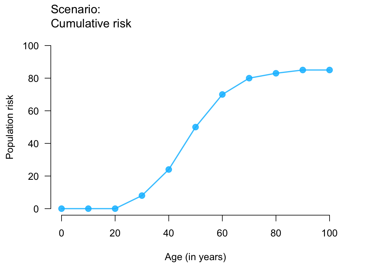
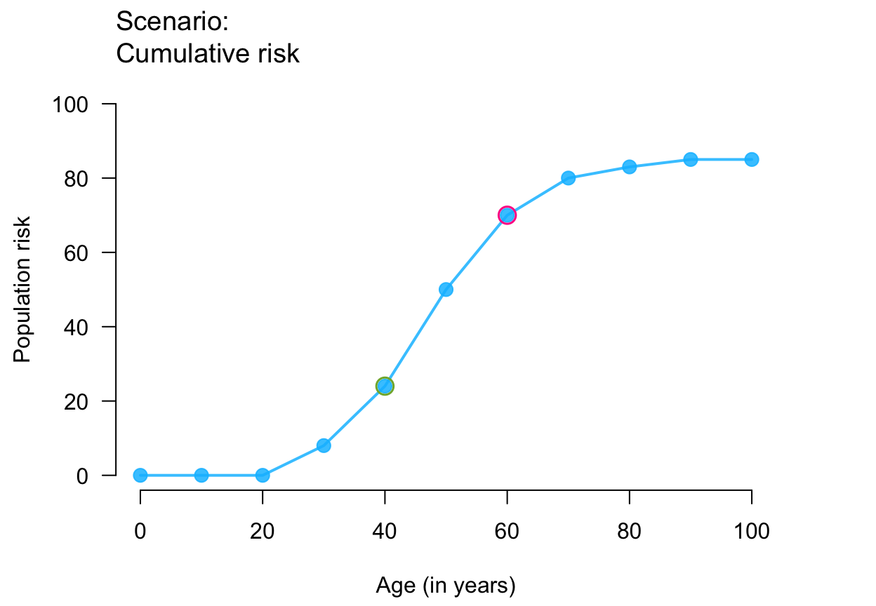
# Data:
x <- seq(0, 100, by = 10)
y <- c(0, 0, 0, 8, 24, 50, 70, 80, 83, 85, 85)
# Basic versions:
plot_crisk(x, y) # using data provided
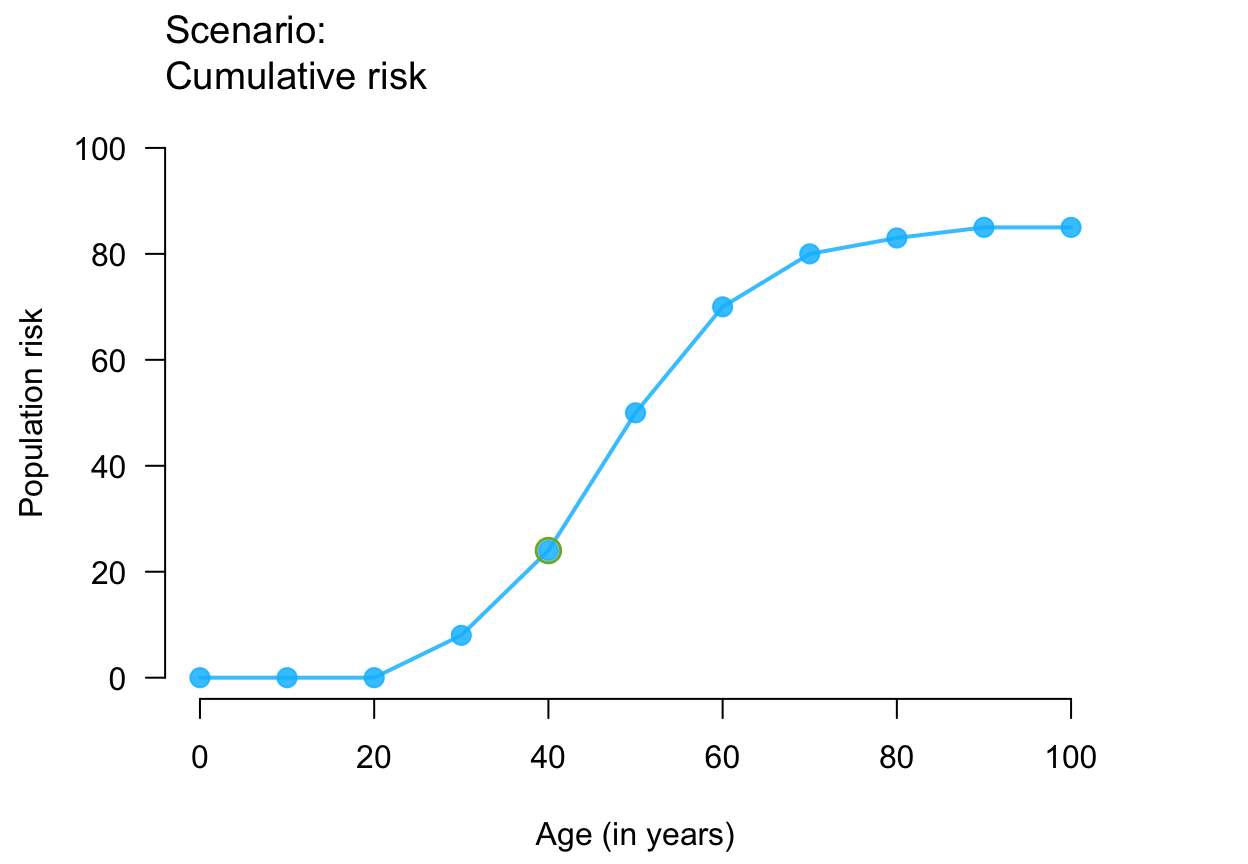
 plot_crisk(x, y, x_from = 40) # use and mark 1 provided point
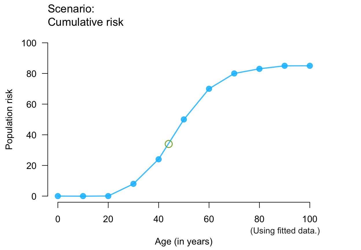
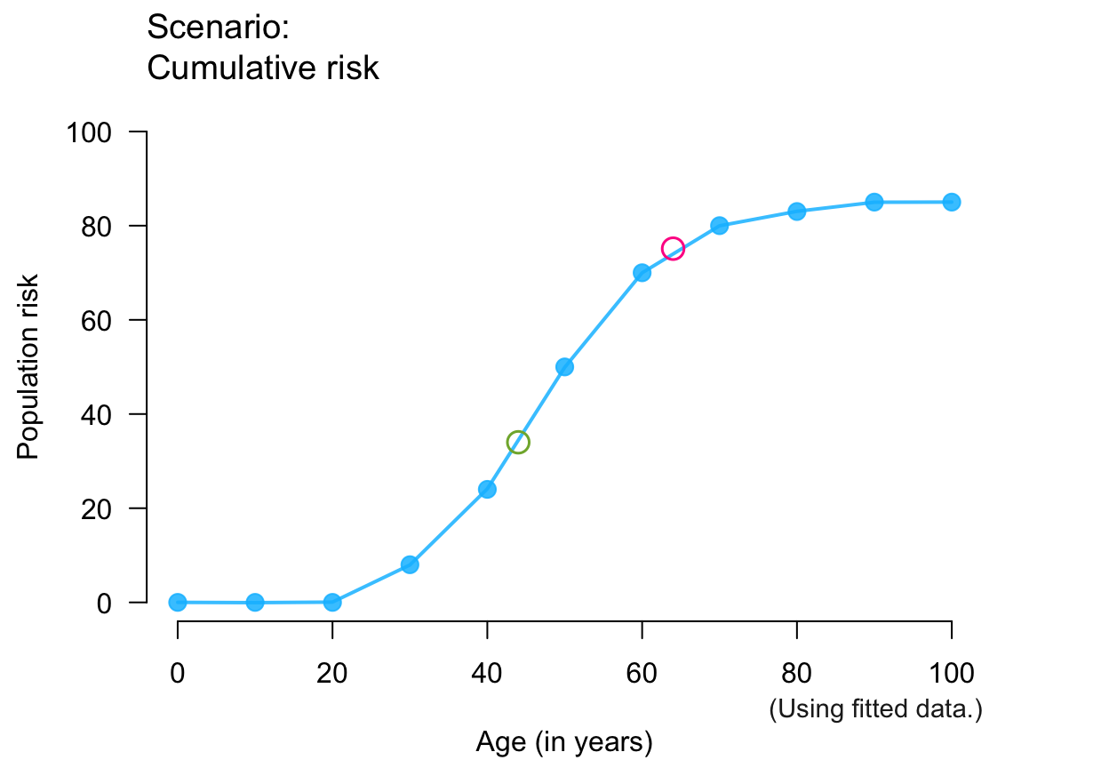
 plot_crisk(x, y, x_from = 44) # use and mark 1 predicted point
#> plot_crisk: x_from is not in x: Using fit_curve = TRUE.
plot_crisk(x, y, x_from = 44) # use and mark 1 predicted point
#> plot_crisk: x_from is not in x: Using fit_curve = TRUE.
 plot_crisk(x, y, x_from = 40, x_to = 60) # use 2 provided points
 plot_crisk(x, y, x_from = 44, x_to = 64) # use 2 predicted points
#> plot_crisk: x_from is not in x: Using fit_curve = TRUE.
plot_crisk(x, y, x_from = 44, x_to = 64) # use 2 predicted points
#> plot_crisk: x_from is not in x: Using fit_curve = TRUE.
 plot_crisk(x, y, fit_curve = TRUE) # fitting curve to provided data
 # Training versions:
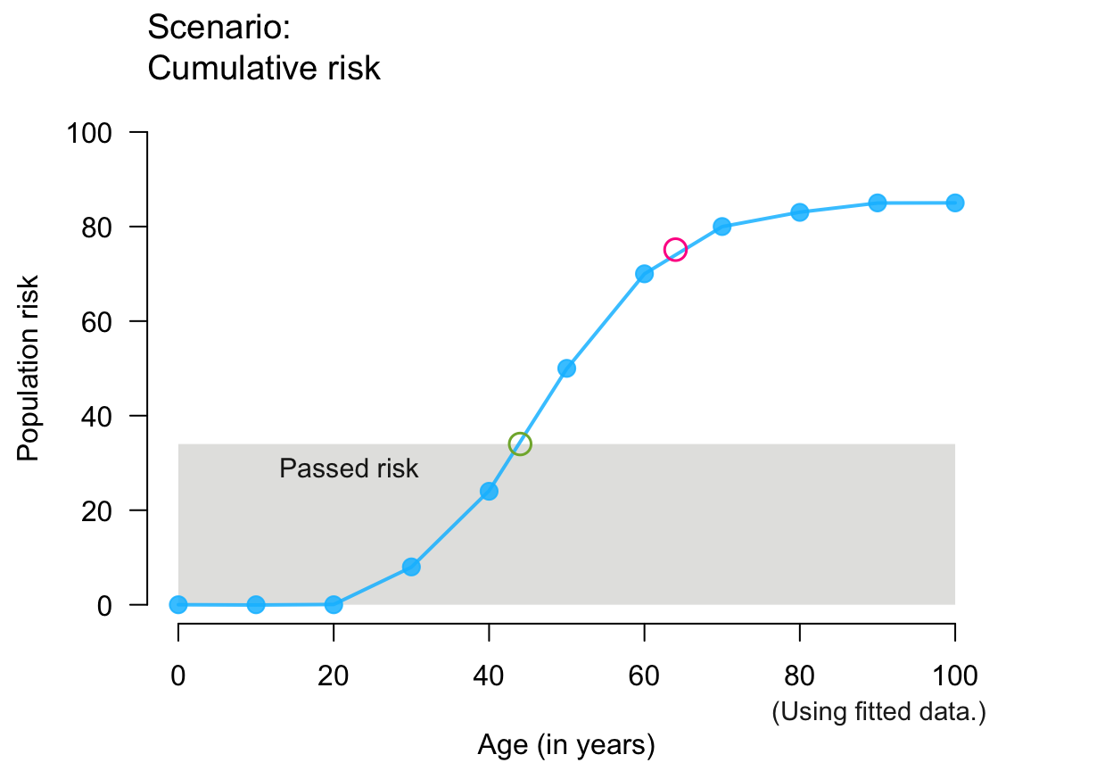
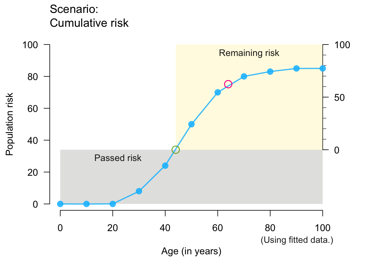
plot_crisk(x, y, 44, 64, show_pas = TRUE) # past/passed risk only
#> plot_crisk: x_from is not in x: Using fit_curve = TRUE.
# Training versions:
plot_crisk(x, y, 44, 64, show_pas = TRUE) # past/passed risk only
#> plot_crisk: x_from is not in x: Using fit_curve = TRUE.
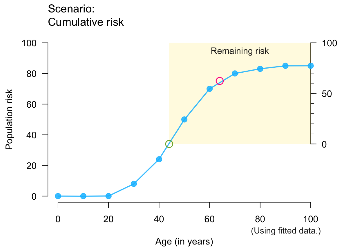
 plot_crisk(x, y, 44, 64, show_rem = TRUE) # remaining risk only
#> plot_crisk: x_from is not in x: Using fit_curve = TRUE.
plot_crisk(x, y, 44, 64, show_rem = TRUE) # remaining risk only
#> plot_crisk: x_from is not in x: Using fit_curve = TRUE.
 plot_crisk(x, y, 44, 64, show_pas = TRUE, show_rem = TRUE) # both risks
#> plot_crisk: x_from is not in x: Using fit_curve = TRUE.
plot_crisk(x, y, 44, 64, show_pas = TRUE, show_rem = TRUE) # both risks
#> plot_crisk: x_from is not in x: Using fit_curve = TRUE.
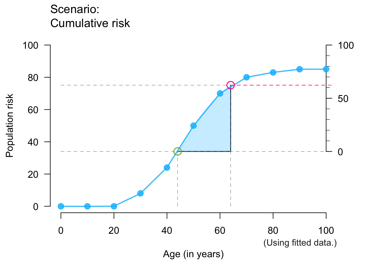
 plot_crisk(x, y, 44, 64, show_aux = TRUE) # auxiliary lines + axis
#> plot_crisk: x_from is not in x: Using fit_curve = TRUE.
plot_crisk(x, y, 44, 64, show_aux = TRUE) # auxiliary lines + axis
#> plot_crisk: x_from is not in x: Using fit_curve = TRUE.
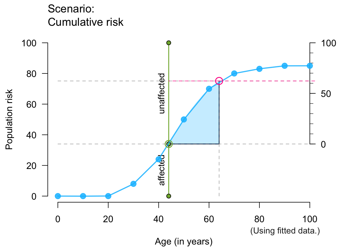
 plot_crisk(x, y, 44, 64, show_aux = TRUE, show_pop = TRUE) # + population parts
#> plot_crisk: x_from is not in x: Using fit_curve = TRUE.
plot_crisk(x, y, 44, 64, show_aux = TRUE, show_pop = TRUE) # + population parts
#> plot_crisk: x_from is not in x: Using fit_curve = TRUE.
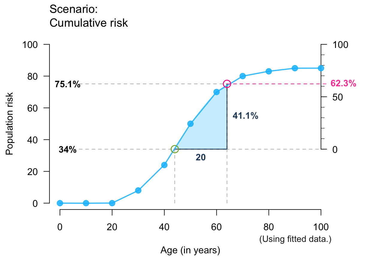
 plot_crisk(x, y, 44, 64, show_aux = TRUE, show_num = TRUE) # + numeric values
#> plot_crisk: x_from is not in x: Using fit_curve = TRUE.
plot_crisk(x, y, 44, 64, show_aux = TRUE, show_num = TRUE) # + numeric values
#> plot_crisk: x_from is not in x: Using fit_curve = TRUE.
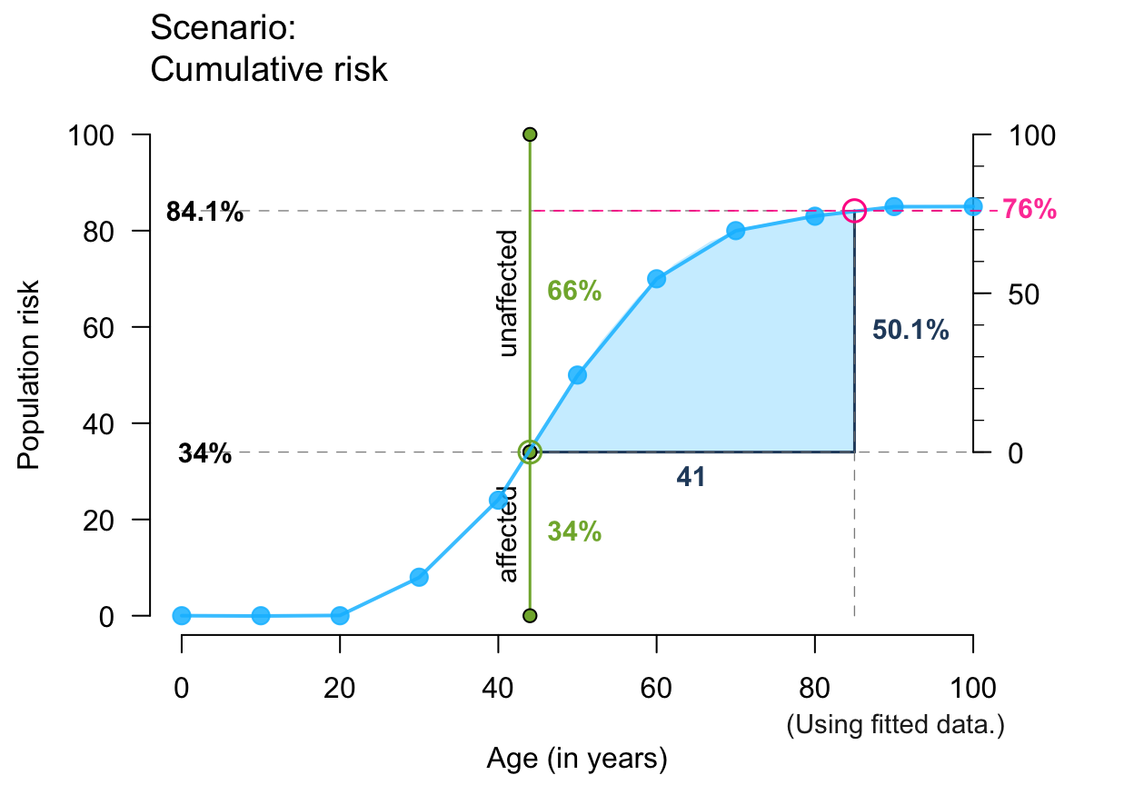
 plot_crisk(x, y, 44, 85, show_aux = TRUE, show_pop = TRUE, show_num = TRUE) # + aux/pop/num
#> plot_crisk: x_from is not in x: Using fit_curve = TRUE.
plot_crisk(x, y, 44, 85, show_aux = TRUE, show_pop = TRUE, show_num = TRUE) # + aux/pop/num
#> plot_crisk: x_from is not in x: Using fit_curve = TRUE.
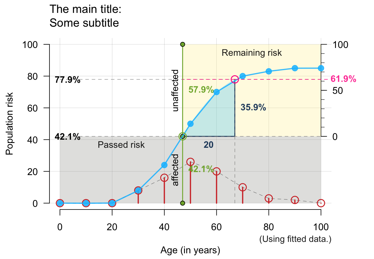
 # Note: Showing ALL is likely to overplot/overwhelm:
plot_crisk(x, y, x_from = 47, x_to = 67, fit_curve = TRUE,
main = "The main title", sub = "Some subtitle",
show_pas = TRUE, show_rem = TRUE, show_aux = TRUE, show_pop = TRUE,
show_num = TRUE, show_inc = TRUE, show_grid = TRUE, mar_notes = TRUE)
# Note: Showing ALL is likely to overplot/overwhelm:
plot_crisk(x, y, x_from = 47, x_to = 67, fit_curve = TRUE,
main = "The main title", sub = "Some subtitle",
show_pas = TRUE, show_rem = TRUE, show_aux = TRUE, show_pop = TRUE,
show_num = TRUE, show_inc = TRUE, show_grid = TRUE, mar_notes = TRUE)
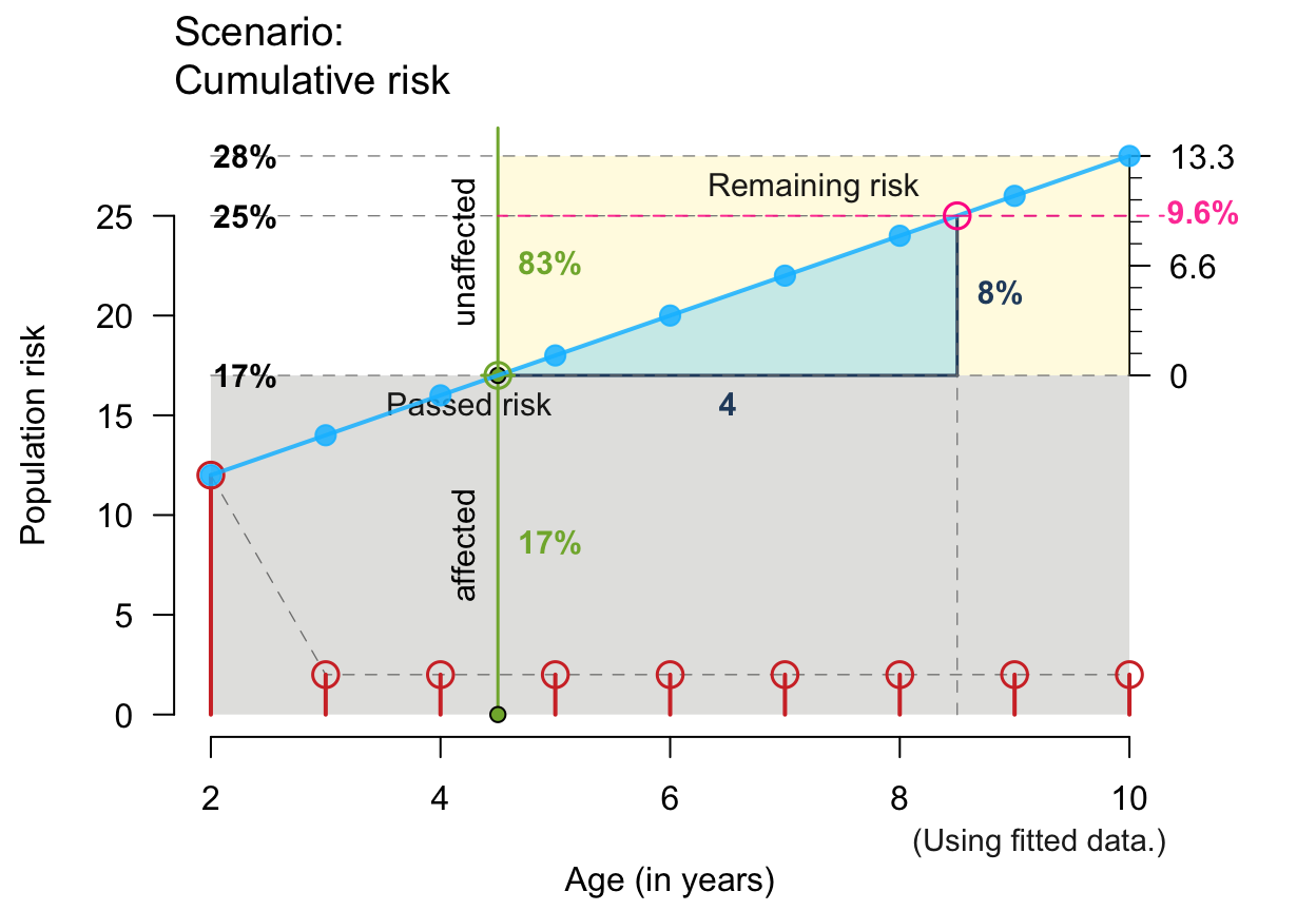
 # Small x- and y-values and linear increases:
plot_crisk(x = 2:10, y = seq(12, 28, by = 2), x_from = 4.5, x_to = 8.5,
show_pas = TRUE, show_rem = TRUE, show_aux = TRUE, show_pop = TRUE,
show_num = TRUE, show_inc = TRUE)
#> plot_crisk: x_from is not in x: Using fit_curve = TRUE.
# Small x- and y-values and linear increases:
plot_crisk(x = 2:10, y = seq(12, 28, by = 2), x_from = 4.5, x_to = 8.5,
show_pas = TRUE, show_rem = TRUE, show_aux = TRUE, show_pop = TRUE,
show_num = TRUE, show_inc = TRUE)
#> plot_crisk: x_from is not in x: Using fit_curve = TRUE.