plot_icons plots a population of which individual's
condition has been classified correctly or incorrectly as icons
from a sufficient and valid set of 3 essential probabilities
(prev, and
sens or its complement mirt, and
spec or its complement fart)
or existing frequency information freq
and a population size of N individuals.
Usage
plot_icons(
  prev = num$prev,
  sens = num$sens,
  mirt = NA,
  spec = num$spec,
  fart = NA,
  N = freq$N,
  sample = FALSE,
  arr_type = "array",
  by = "all",
  ident_order = c("hi", "mi", "fa", "cr"),
  icon_types = 22,
  icon_size = NULL,
  icon_brd_lwd = 1.5,
  block_d = NULL,
  border_d = 0.1,
  block_size_row = 10,
  block_size_col = 10,
  nblocks_row = NULL,
  nblocks_col = NULL,
  fill_array = "left",
  fill_blocks = "rowwise",
  lbl_txt = txt,
  main = txt$scen_lbl,
  sub = "type",
  title_lbl = NULL,
  cex_lbl = 0.9,
  col_pal = pal,
  transparency = 0.5,
  mar_notes = FALSE,
  ...
)
Arguments
- prev
The condition's prevalence
prev(i.e., the probability of condition beingTRUE).- sens
The decision's sensitivity
sens(i.e., the conditional probability of a positive decision provided that the condition isTRUE).sensis optional when its complementmirtis provided.- mirt
The decision's miss rate
mirt(i.e., the conditional probability of a negative decision provided that the condition isTRUE).mirtis optional when its complementsensis provided.- spec
The decision's specificity value
spec(i.e., the conditional probability of a negative decision provided that the condition isFALSE).specis optional when its complementfartis provided.- fart
The decision's false alarm rate
fart(i.e., the conditional probability of a positive decision provided that the condition isFALSE).fartis optional when its complementspecis provided.- N
The number of individuals in the population. A suitable value of
Nis computed, if not provided. If N is 100,000 or greater it is reduced to 10,000 for the array types if the frequencies allow it.- sample
Boolean value that determines whether frequency values are sampled from
N, given the probability values ofprev,sens, andspec. Default:sample = FALSE.- arr_type
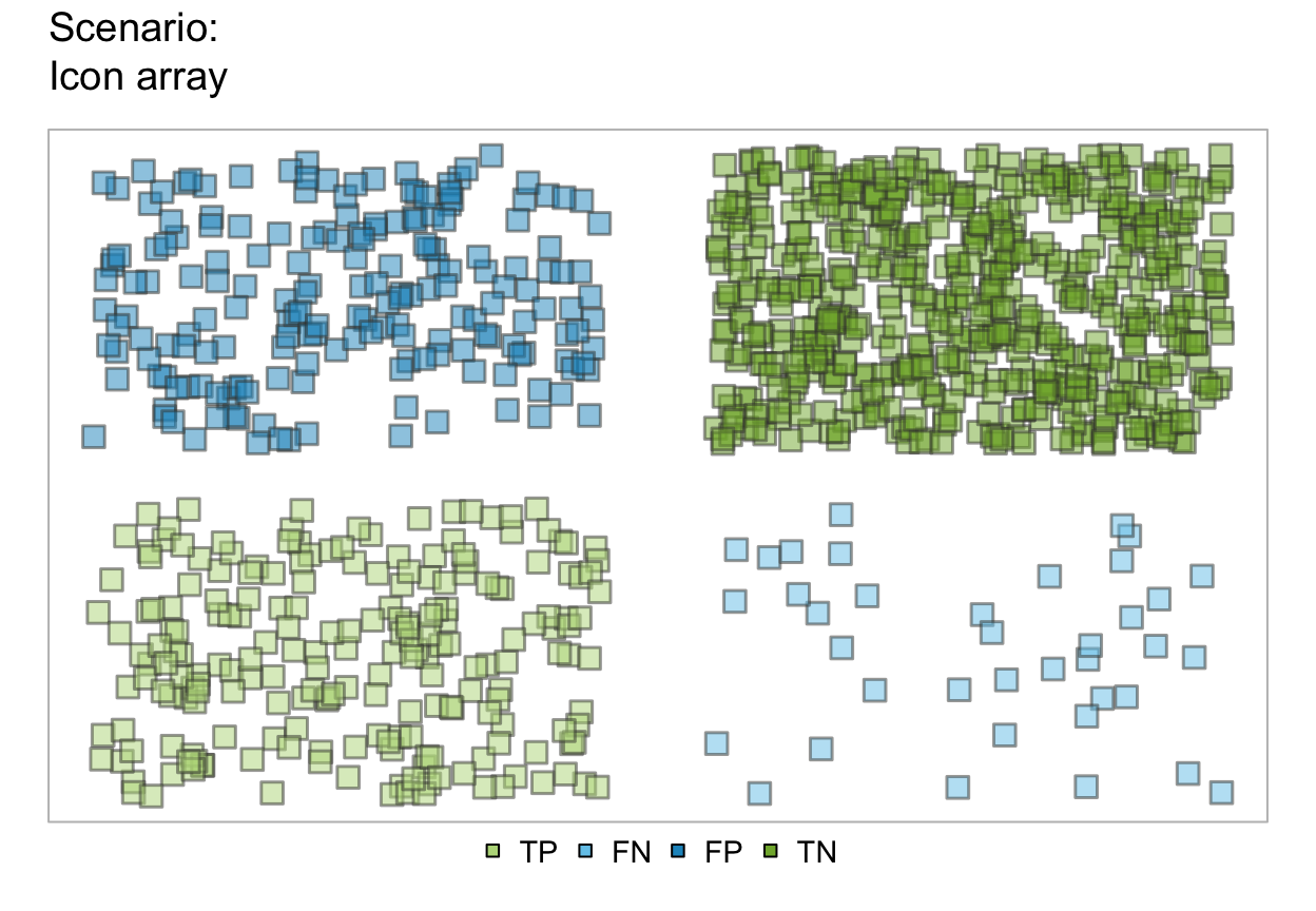
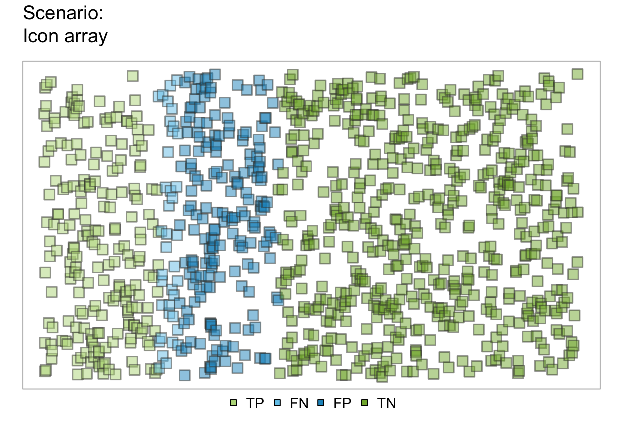
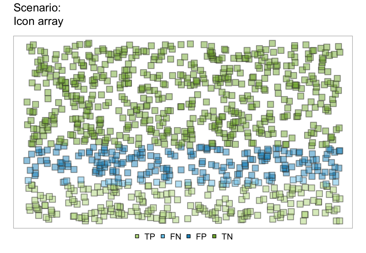
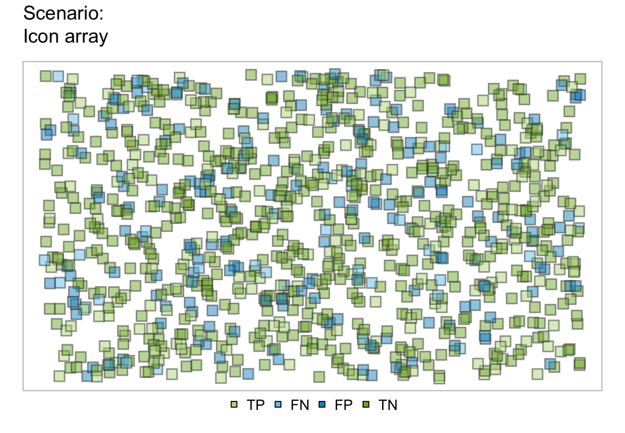
The icons can be arranged in different ways resulting in different types of displays:
arr_type = "array": Icons are plotted in a classical icon array (default). Icons can be arranged in blocks usingblock_d. The order of filling the array can be customized usingfill_arrayandfill_blocks.arr_type = "shuffledarray": Icons are plotted in an icon array, but positions are shuffled (randomized). Icons can be arranged in blocks usingblock_d. The order of filling the array can be customized usingfill_arrayandfill_blocks.arr_type = "mosaic": Icons are ordered like in a mosaic plot. The area size displays the relative proportions of their frequencies.arr_type = "fillequal": Icons are positioned into equally sized blocks. Thus, their density reflects the relative proportions of their frequencies.arr_type = "fillleft": Icons are randomly filled from the left.arr_type = "filltop": Icons are randomly filled from the top.arr_type = "scatter": Icons are randomly scattered into the plot.
- by
A character code specifying a perspective to split the population into subsets, with 4 options:
- ident_order
The order in which icon identities (i.e., hi, mi, fa, and cr) are plotted. Default:
ident_order = c("hi", "mi", "fa", "cr")- icon_types
specifies the appearance of the icons as a vector. Default:
icon_types = 11(i.e., squares with border). Accepts values from 1 to 25 (see?points).- icon_size
specifies the size of the icons via
cexDefault:icon_size = NULLfor automatic calculation.- icon_brd_lwd
specifies the border width of icons (if applicable). Default:
icon_brd_lwd = 1.5. Set toNAfor no border.- block_d
The distance between blocks. Default:
block_d = NULLfor automatic calculation; (does not apply to "filleft", "filltop", and "scatter")- border_d
The distance of icons to the border. Default:
border_d = 0.1.Additional options for controlling the arrangement of arrays (for
arr_type = "array"and"shuffledarray"):- block_size_row
specifies how many icons should be in each block row. Default:
block_size_row = 10.- block_size_col
specifies how many icons should be in each block column. Default:
block_size_col = 10.- nblocks_row
Number of blocks per row. Default:
nblocks_row = NULLfor automatic calculation.- nblocks_col
Number of blocks per column. Default:
nblocks_col = NULLfor automatic calculation.- fill_array
specifies how the blocks are filled into the array. Options:
fill_array = "left"(default) vs."top".- fill_blocks
specifies how icons within blocks are filled. Options:
fill_blocks = "rowwise"(default) and"colwise".Generic text and color options:
- lbl_txt
Default label set for text elements. Default:
lbl_txt = txt.- main
Text label for main plot title. Default:
main = txt$scen_lbl.- sub
Text label for plot subtitle (on 2nd line). Default:
sub = "type"shows information on current plot type.- title_lbl
Deprecated text label for current plot title. Replaced by
main.- cex_lbl
Scaling factor for text labels. Default:
cex_lbl = .90.- col_pal
Color palette. Default:
col_pal = pal.- transparency
Specifies the transparency for overlapping icons (not for
arr_type = "array"and"shuffledarray").- mar_notes
Boolean option for showing margin notes. Default:
mar_notes = FALSE.- ...
Other (graphical) parameters.
Details
If probabilities are provided, a new list of
natural frequencies freq is computed by comp_freq.
By contrast, if no probabilities are provided,
the values currently contained in freq are used.
By default, comp_freq rounds frequencies to nearest integers
to avoid decimal values in freq.
See also
Other visualization functions:
plot.riskyr(),
plot_area(),
plot_bar(),
plot_crisk(),
plot_curve(),
plot_fnet(),
plot_mosaic(),
plot_plane(),
plot_prism(),
plot_tab(),
plot_tree()
Examples
# Basics:
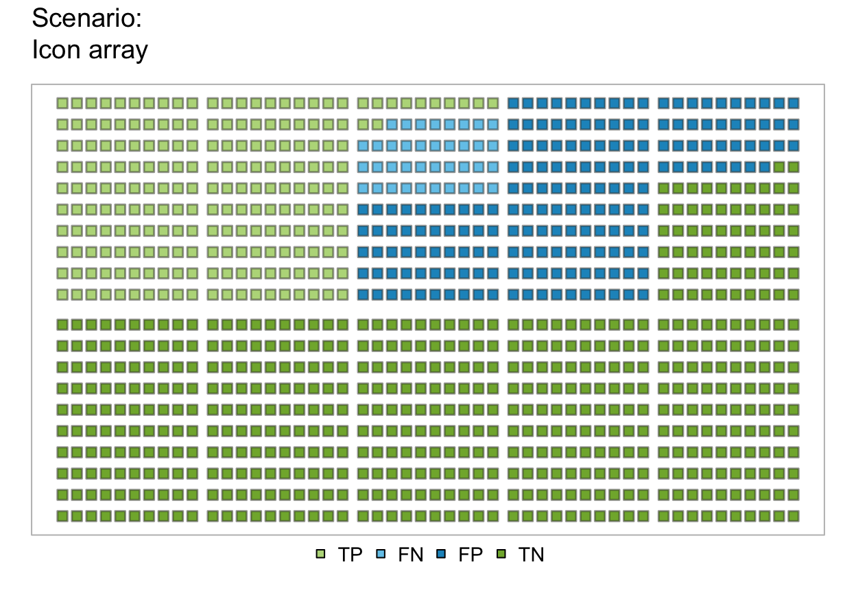
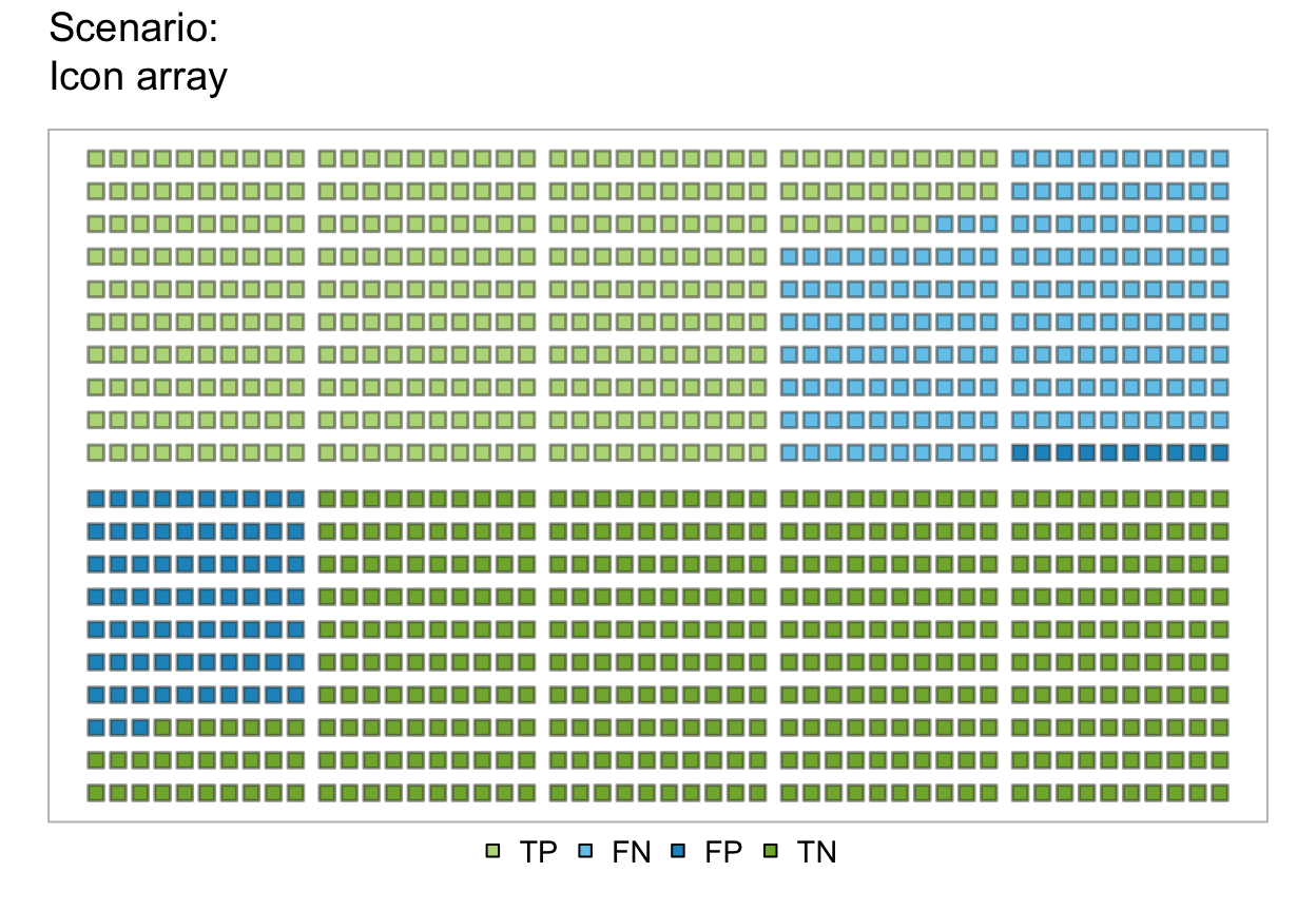
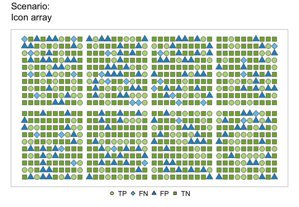
plot_icons(N = 1000) # icon array with default settings (arr_type = "array")
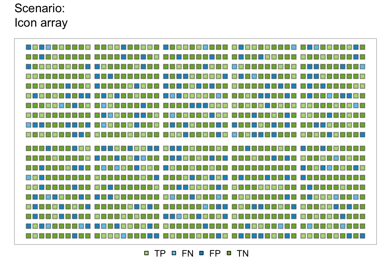
 plot_icons(arr_type = "shuffledarray", N = 1000) # icon array with shuffled IDs
 # Sampling:
plot_icons(N = 1000, prev = 1/2, sens = 2/3, spec = 6/7, sample = TRUE)
# Sampling:
plot_icons(N = 1000, prev = 1/2, sens = 2/3, spec = 6/7, sample = TRUE)
 # array types:
plot_icons(arr_type = "mosaic", N = 1000) # areas as in mosaic plot
# array types:
plot_icons(arr_type = "mosaic", N = 1000) # areas as in mosaic plot
 plot_icons(arr_type = "fillequal", N = 1000) # areas of equal size (probability as density)
 plot_icons(arr_type = "fillleft", N = 1000) # icons filled from left to right (in columns)
 plot_icons(arr_type = "filltop", N = 1000) # icons filled from top to bottom (in rows)
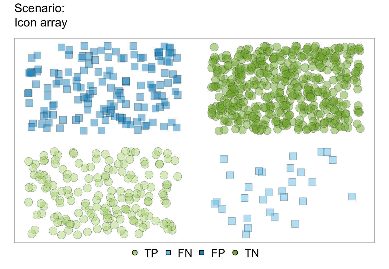
 plot_icons(arr_type = "scatter", N = 1000) # icons randomly scattered
 # by:
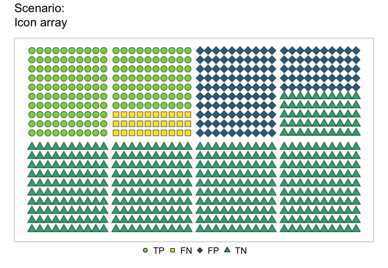
plot_icons(N = 1000, by = "all") # hi, mi, fa, cr (TP, FN, FP, TN) cases
# by:
plot_icons(N = 1000, by = "all") # hi, mi, fa, cr (TP, FN, FP, TN) cases
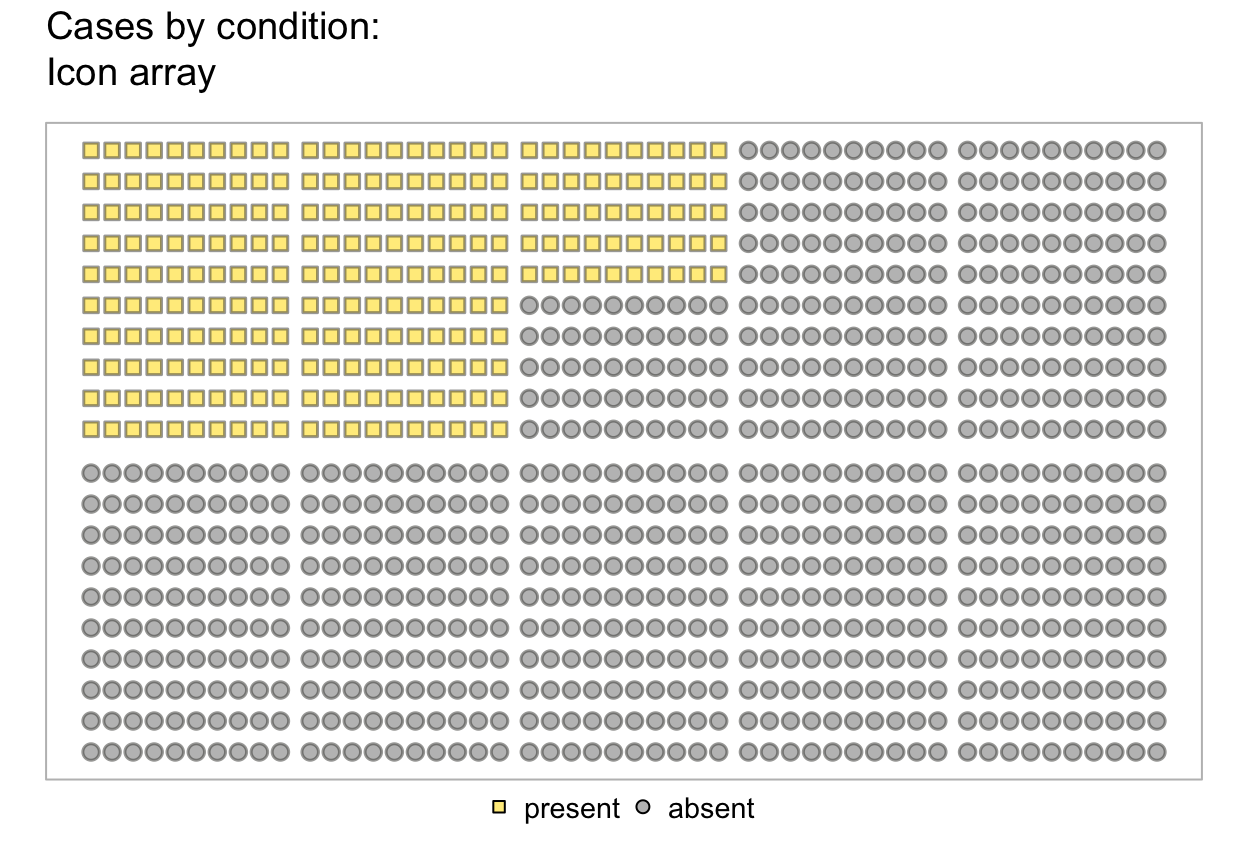
 plot_icons(N = 1000, by = "cd", main = "Cases by condition") # (hi + mi) vs. (fa + cr)
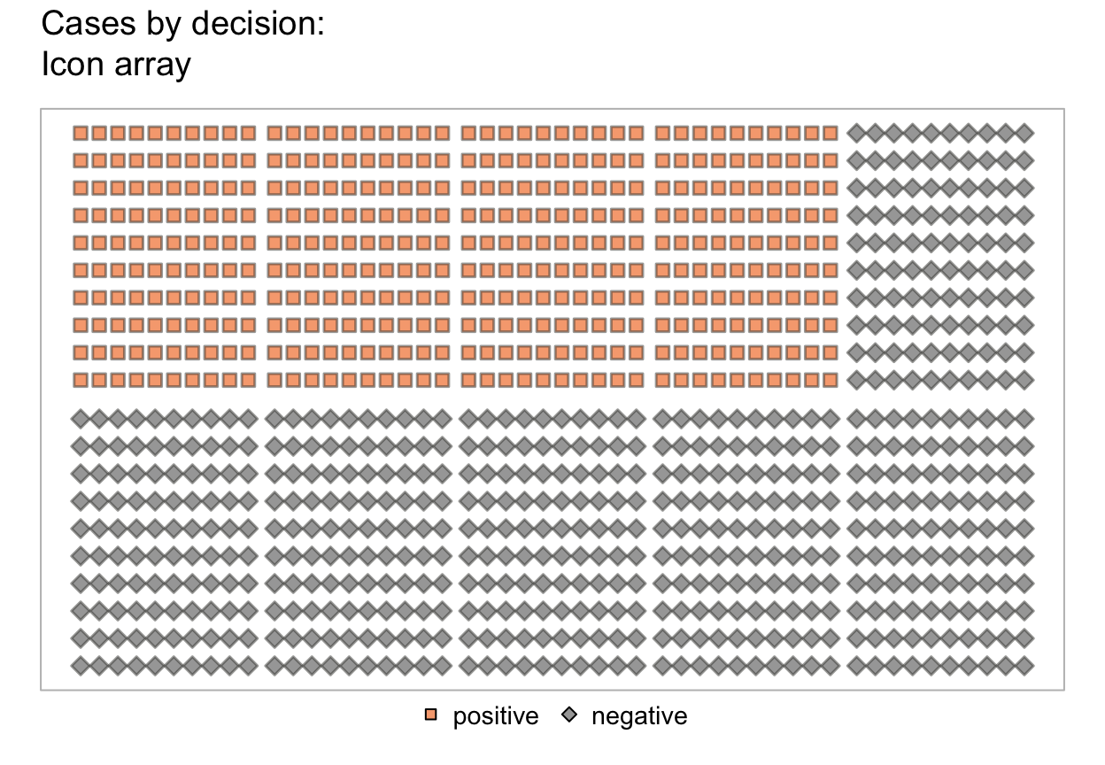
 plot_icons(N = 1000, by = "dc", main = "Cases by decision") # (hi + fa) vs. (mi + cr)
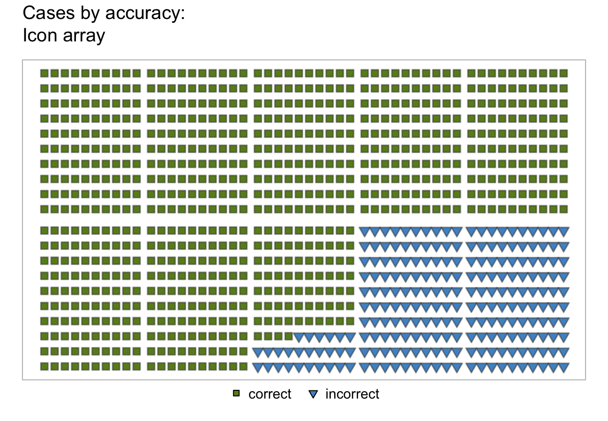
 plot_icons(N = 1000, by = "ac", main = "Cases by accuracy") # (hi + cr) vs. (fa + mi)
 # Custom icon types and colors:
plot_icons(N = 800, arr_type = "array", icon_types = c(21, 22, 23, 24),
block_d = 0.5, border_d = 0.5, col_pal = pal_vir)
# Custom icon types and colors:
plot_icons(N = 800, arr_type = "array", icon_types = c(21, 22, 23, 24),
block_d = 0.5, border_d = 0.5, col_pal = pal_vir)
 plot_icons(N = 800, arr_type = "shuffledarray", icon_types = c(21, 23, 24, 22),
block_d = 0.5, border_d = 0.5)
plot_icons(N = 800, arr_type = "shuffledarray", icon_types = c(21, 23, 24, 22),
block_d = 0.5, border_d = 0.5)
 plot_icons(N = 800, arr_type = "fillequal", icon_types = c(21, 22, 22, 21),
icon_brd_lwd = .5, cex = 1, cex_lbl = 1.1)
plot_icons(N = 800, arr_type = "fillequal", icon_types = c(21, 22, 22, 21),
icon_brd_lwd = .5, cex = 1, cex_lbl = 1.1)
 # Text and color options:
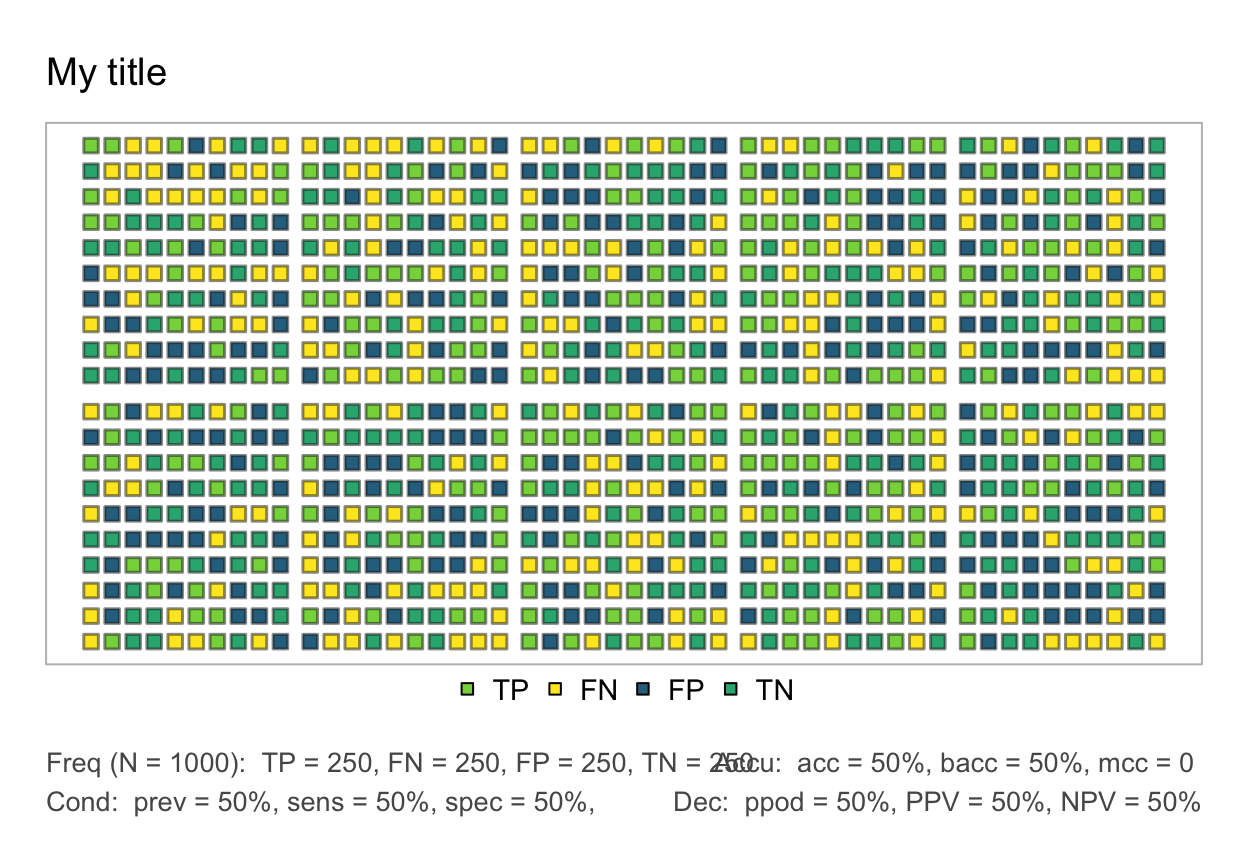
plot_icons(N = 1000, prev = .5, sens = .5, spec = .5, arr_type = "shuffledarray",
main = "My title", sub = NA, lbl_txt = txt_TF, col_pal = pal_vir, mar_notes = TRUE)
# Text and color options:
plot_icons(N = 1000, prev = .5, sens = .5, spec = .5, arr_type = "shuffledarray",
main = "My title", sub = NA, lbl_txt = txt_TF, col_pal = pal_vir, mar_notes = TRUE)
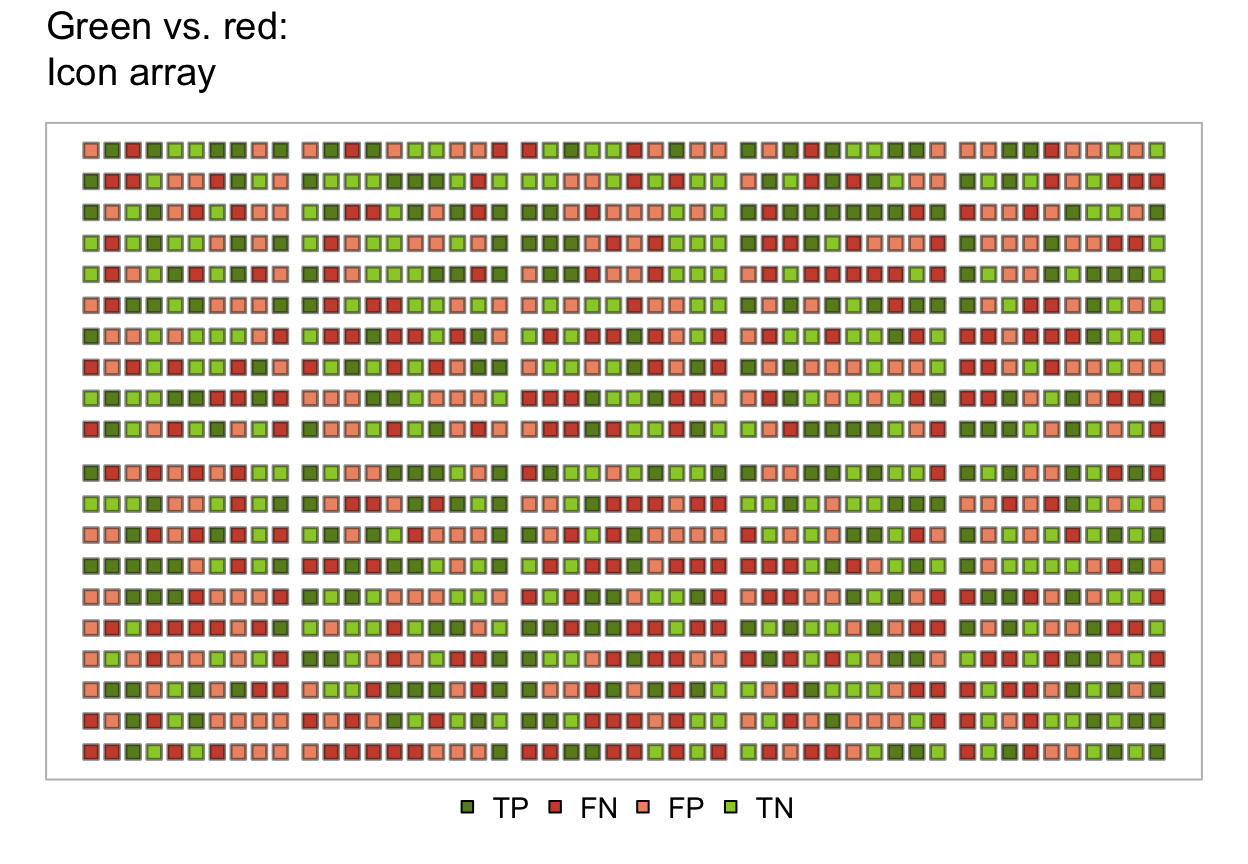
 plot_icons(N = 1000, prev = .5, sens = .5, spec = .5, arr_type = "shuffledarray",
main = "Green vs. red", col_pal = pal_rgb, transparency = .5)
plot_icons(N = 1000, prev = .5, sens = .5, spec = .5, arr_type = "shuffledarray",
main = "Green vs. red", col_pal = pal_rgb, transparency = .5)