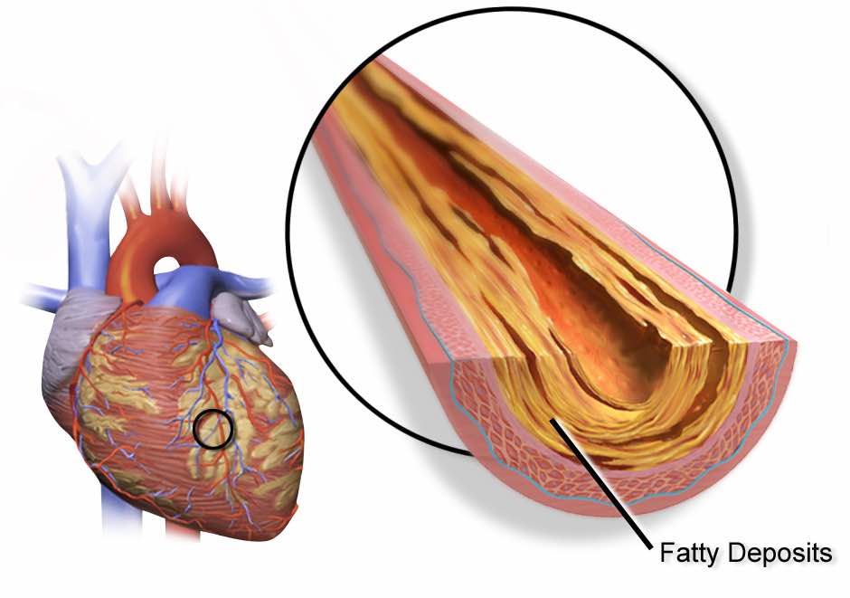
Creating FFTs with FFTrees()

Details on the `FFTrees()` function

This vignette starts by building a fast-and-frugal tree (FFT) from the heartdisease data — also used in the Tutorial: FFTs for heart disease and Phillips et al. (2017) — but then explores additional aspects of the FFTrees() function.

The goal of the FFTrees() function is to create FFTs from data and record all details of the problem specification, tree definitions, the classification process, and performance measures in an FFTrees object. As FFTrees() can handle two sets of data (for training vs. testing) and creates a range of FFTs, each with distinct process and performance characteristics, evaluating the function may take some time (typically a few seconds) and the structure of the resulting FFTrees object is quite complex. But as FFTrees() is at the heart of the FFTrees package, it pays to understand its arguments and the structure of an FFTrees object.

Example: Predicting heart disease

An FFT generally addresses binary classification problems: It attempts to classify the outcomes of a criterion variable into one of two classes (i.e., True or False) based on a range of potential predictor variables (aka. cues or features). A corresponding problem from the domain of clinical diagnostics is:

Which patient has heart disease, given some data on patients’ general health and diagnostic symptoms?

To address this problem, the FFTrees package includes the heartdisease data. But rather than using the full dataset to fit our FFTs, we have split the data into a training set (heart.train), and test set (heart.test). Here is a peak at the corresponding data frames:

# Training data: 
head(heart.train)

#> # A tibble: 6 × 14
#>   diagnosis   age   sex cp    trestbps  chol   fbs restecg thalach exang oldpeak
#>   <lgl>     <dbl> <dbl> <chr>    <dbl> <dbl> <dbl> <chr>     <dbl> <dbl>   <dbl>
#> 1 FALSE        44     0 np         108   141     0 normal      175     0     0.6
#> 2 FALSE        51     0 np         140   308     0 hypert…     142     0     1.5
#> 3 FALSE        52     1 np         138   223     0 normal      169     0     0  
#> 4 TRUE         48     1 aa         110   229     0 normal      168     0     1  
#> 5 FALSE        59     1 aa         140   221     0 normal      164     1     0  
#> 6 FALSE        58     1 np         105   240     0 hypert…     154     1     0.6
#> # ℹ 3 more variables: slope <chr>, ca <dbl>, thal <chr>

# Testing data:
head(heart.test)

#> # A tibble: 6 × 14
#>   diagnosis   age   sex cp    trestbps  chol   fbs restecg thalach exang oldpeak
#>   <lgl>     <dbl> <dbl> <chr>    <dbl> <dbl> <dbl> <chr>     <dbl> <dbl>   <dbl>
#> 1 FALSE        51     0 np         120   295     0 hypert…     157     0     0.6
#> 2 TRUE         45     1 ta         110   264     0 normal      132     0     1.2
#> 3 TRUE         53     1 a          123   282     0 normal       95     1     2  
#> 4 TRUE         45     1 a          142   309     0 hypert…     147     1     0  
#> 5 FALSE        66     1 a          120   302     0 hypert…     151     0     0.4
#> 6 TRUE         48     1 a          130   256     1 hypert…     150     1     0  
#> # ℹ 3 more variables: slope <chr>, ca <dbl>, thal <chr>

The critical dependent variable (or binary criterion variable) is diagnosis. This variable indicates whether a patient has heart disease (diagnosis = TRUE) or not (diagnosis = FALSE). All other variables in the dataset (e.g., sex, age, and several biological measurements) can be used as predictors (aka. cues).

Creating trees with `FFTrees()`

To illustrate the difference between fitting and prediction, we will train the FFTs on heart.train, and test their prediction performance in heart.test. Note that we can also automate the training / test split using the train.p argument in FFTrees(). Setting train.p will randomly split train.p% of the original data into a training set.

To create a set of FFTs, we use the FFTrees() function to create a new FFTrees object called heart.fft. Here, we specify diagnosis as the binary criterion (or dependent variable), and include all other (independent) variables with formula = diagnosis ~ .:

# Create an FFTrees object called heart.fft predicting diagnosis: 
heart.fft <- FFTrees(formula = diagnosis ~.,
                     data = heart.train,
                     data.test = heart.test)

If we wanted to only consider specific variables, like sex and age, for our trees, we could specify formula = diagnosis ~ age + sex.

Elements of an `FFTrees` object

The FFTrees() function returns an object of the FFTrees class. There are many elements in an FFTrees object. We can obtain these elements by printing their names:

# See the elements of an FFTrees object:
names(heart.fft)

#> [1] "criterion_name" "cue_names"      "formula"        "trees"         
#> [5] "data"           "params"         "competition"    "cues"

Inspecting these elements provides a wealth of information on the range of FFTs contained in the current FFTrees object:

criterion_name: The name of the (predicted) binary criterion variable.
cue_names: The names of all potential cue variables (predictors) in the data.
formula: The formula used to create the FFTrees object.
trees: Information on all trees contained in the object, with list elements that specify their number n, the best tree, as well as tree definitions, verbal descriptions (inwords), decisions, and the performance characteristics (stats and level_stats) of each FFT.
data: The datasets used to train and test the FFTs (if applicable).
params: The parameters used for constructing FFTs (currently 19 parameters).
competition: Models and statistics of alternative classification algorithms (for test, train, and models).
cues: Information on all cue variables (predictors), with list elements that specify their thresholds and performance stats when training FFTs.

Basic performance characteristics of FFTs

We can view basic information about the FFTrees object by printing its name. As the default tree construction algorithm ifan creates multiple trees with different exit structures, an FFTrees object typically contains many FFTs.

When printing an FFTrees object, we automatically see the performance on the training data (i.e., for fitting, rather than prediction) and obtain the information about the tree with the highest value of the goal statistic. By default, the goal is set to weighed accuracy wacc:

# Training performance of the best tree (on "train" data, given current goal):
heart.fft  # same as: print(heart.fft, data = "train")

#> FFTrees 
#> - Trees: 7 fast-and-frugal trees predicting diagnosis
#> - Cost of outcomes:  hi = 0,  fa = 1,  mi = 1,  cr = 0
#> - Cost of cues: 
#>      age      sex       cp trestbps     chol      fbs  restecg  thalach 
#>        1        1        1        1        1        1        1        1 
#>    exang  oldpeak    slope       ca     thal 
#>        1        1        1        1        1 
#> 
#> FFT #1: Definition
#> [1] If thal = {rd,fd}, decide True.
#> [2] If cp != {a}, decide False.
#> [3] If ca > 0, decide True, otherwise, decide False.
#> 
#> FFT #1: Training Accuracy
#> Training data: N = 150, Pos (+) = 66 (44%) 
#> 
#> |          | True + | True - | Totals:
#> |----------|--------|--------|
#> | Decide + | hi  54 | fa  18 |      72
#> | Decide - | mi  12 | cr  66 |      78
#> |----------|--------|--------|
#>   Totals:        66       84   N = 150
#> 
#> acc  = 80.0%   ppv  = 75.0%   npv  = 84.6%
#> bacc = 80.2%   sens = 81.8%   spec = 78.6%
#> 
#> FFT #1: Training Speed, Frugality, and Cost
#> mcu = 1.74,  pci = 0.87
#> cost_dec = 0.200,  cost_cue = 1.740,  cost = 1.940

Before interpreting any model output, we need to carefully distinguish between an FFT’s “Training” (for fitting training data) and “Prediction” performance (for new test data). Unless we explicitly ask for print(heart.fft, data = "test"), the output of printing heart.fft will report on the fitting phase (i.e., data = "train" by default). To see the corresponding prediction performance, we could alternatively ask for:

# Prediction performance of the best training tree (on "test" data): 
print(heart.fft, data = "test")

When evaluating an FFT for either training or test data, we obtain a wide range of measures.

After some general information on the FFTrees object, we see a verbal Definition of the best FFT (FFT #1). Key information for evaluating an FFT’s performance is contained in the Accuracy panel (for either training or prediction). Here is a description of the frequency counts and corresponding statistics provided:

Statistic	Long name	Definition
Frequencies:
`hi`	Number of hits	$N(\text{Decision} = 1 \land \text{Truth} = 1)$
`mi`	Number of misses	$N(\text{Decision} = 0 \land \text{Truth} = 1)$
`fa`	Number of false-alarms	$N(\text{Decision} = 1 \land \text{Truth} = 0)$
`cr`	Number of correct rejections	$N(\text{Decision} = 0 \land \text{Truth} = 0)$
`N`	Number of cases	The total number of cases considered.
Probabilities:
`acc`	Accuracy	The percentage of cases that were correctly classified.
`ppv`	Positive predictive value	The percentage (or conditional probability) of positive decisions being correct (i.e., True + cases).
`npv`	Negative predictive value	The percentage (or conditional probability) of negative decisions being correct (i.e., True - cases).
`wacc`	Weighted accuracy	The weighted average of sensitivity and specificity, where sensitivity is weighted by `sens.w` (by default, `sens.w = .50`).
`sens`	Sensitivity	The percentage (or conditional probability) of true positive cases being correctly classified.
`spec`	Specificity	The percentage (or conditional probability) of true negative cases being correctly classified.
Frugality:
`mcu`	Mean cues used	On average, how many cues were needed to classify cases? In other words, what percent of the available information was used on average?
`pci`	Percent cues ignored	The percent of data that was ignored when classifying cases with a given tree. This is identical to `mcu / cues.n`, where `cues.n` is the total number of cues in the data.

Table 1: Description of FFTs’ basic frequencies and corresponding accuracy and speed/frugality statistics.

To obtain the same information for another FFT of an FFTrees object, we can call print() with a numeric tree parameter. For instance, the following expression would provide the basic performance characteristics of Tree 3:

# Performance of alternative FFTs (Tree 3) in an FFTrees object: 
print(heart.fft, tree = 3, data = "test")

Alternatively, we could visualize the same tree and its performance characteristics by calling plot(heart.fft, tree = 3, data = "test").

See the Accuracy statistics vignette for details on the accuracy statistics used throughout the FFTrees package.

Cue performance information

Each FFT has a decision threshold for each cue (regardless of whether or not it is actually used in the tree) that maximizes the goal value of that cue when it is applied to the entire training dataset. We can obtain cue accuracy statistics using the calculated decision thresholds from the cue.accuracies list. If the object has test data, we can see the marginal cue accuracies in the test data (using the thresholds calculated from the training data):

# Decision thresholds and marginal classification training accuracies for each cue: 
heart.fft$cues$stats$train

#>         cue     class            threshold direction   n hi fa mi cr      sens
#> 1       age   numeric                   57         > 150 38 22 28 62 0.5757576
#> 2       sex   numeric                    0         > 150 53 48 13 36 0.8030303
#> 3        cp character                    a         = 150 48 18 18 66 0.7272727
#> 4  trestbps   numeric                  148         > 150 15  9 51 75 0.2272727
#> 5      chol   numeric                  273         > 150 22 17 44 67 0.3333333
#> 6       fbs   numeric                    0         > 150 10  9 56 75 0.1515152
#> 7   restecg character hypertrophy,abnormal         = 150 40 34 26 50 0.6060606
#> 8   thalach   numeric                  154        <= 150 44 29 22 55 0.6666667
#> 9     exang   numeric                    0         > 150 31 14 35 70 0.4696970
#> 10  oldpeak   numeric                  0.8         > 150 41 22 25 62 0.6212121
#> 11    slope character            flat,down         = 150 45 27 21 57 0.6818182
#> 12       ca   numeric                    0         > 150 47 19 19 65 0.7121212
#> 13     thal character                rd,fd         = 150 47 16 19 68 0.7121212
#>         spec       ppv       npv       acc      bacc      wacc    dprime
#> 1  0.7380952 0.6333333 0.6888889 0.6666667 0.6569264 0.6569264 0.8227611
#> 2  0.4285714 0.5247525 0.7346939 0.5933333 0.6158009 0.6158009 0.6653742
#> 3  0.7857143 0.7272727 0.7857143 0.7600000 0.7564935 0.7564935 1.3853056
#> 4  0.8928571 0.6250000 0.5952381 0.6000000 0.5600649 0.5600649 0.4882880
#> 5  0.7976190 0.5641026 0.6036036 0.5933333 0.5654762 0.5654762 0.3996338
#> 6  0.8928571 0.5263158 0.5725191 0.5666667 0.5221861 0.5221861 0.2105078
#> 7  0.5952381 0.5405405 0.6578947 0.6000000 0.6006494 0.6006494 0.5065806
#> 8  0.6547619 0.6027397 0.7142857 0.6600000 0.6607143 0.6607143 0.8230087
#> 9  0.8333333 0.6888889 0.6666667 0.6733333 0.6515152 0.6515152 0.8840984
#> 10 0.7380952 0.6507937 0.7126437 0.6866667 0.6796537 0.6796537 0.9394337
#> 11 0.6785714 0.6250000 0.7307692 0.6800000 0.6801948 0.6801948 0.9297212
#> 12 0.7738095 0.7121212 0.7738095 0.7466667 0.7429654 0.7429654 1.3009993
#> 13 0.8095238 0.7460317 0.7816092 0.7666667 0.7608225 0.7608225 1.4243467
#>      cost_dec      cost cost_cue
#> 1  -0.3333333 -1.333333        1
#> 2  -0.4066667 -1.406667        1
#> 3  -0.2400000 -1.240000        1
#> 4  -0.4000000 -1.400000        1
#> 5  -0.4066667 -1.406667        1
#> 6  -0.4333333 -1.433333        1
#> 7  -0.4000000 -1.400000        1
#> 8  -0.3400000 -1.340000        1
#> 9  -0.3266667 -1.326667        1
#> 10 -0.3133333 -1.313333        1
#> 11 -0.3200000 -1.320000        1
#> 12 -0.2533333 -1.253333        1
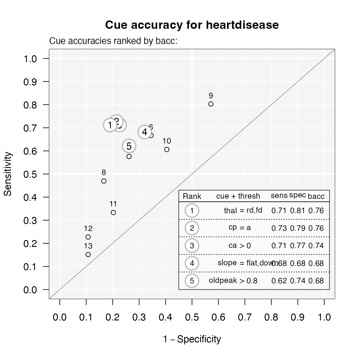
#> 13 -0.2333333 -1.233333        1

We can also visualize the cue accuracies for the training data (in ROC space, i.e., showing each cue’s hit rate by its false alarm rate) by calling plot() with the what = "cues" argument. This will show the sensitivities and specificities for each cue, with the top five cues highlighted and listed:

# Visualize individual cue accuracies: 
plot(heart.fft, what = "cues", 
     main = "Cue accuracy for heartdisease")

#> Plotting cue training statistics:
#> — Cue accuracies ranked by bacc
#>

See the Plotting FFTrees objects vignette for more details on visualizing cue accuracies and FFTs.

Tree definitions

The tree.definitions data frame contains definitions (cues, classes, exits, thresholds, and directions) of all trees in an FFTrees object. The combination of these five pieces of information (as well as their order), define and describe how a tree makes decisions:

# See the definitions of all trees:
heart.fft$trees$definitions

#> # A tibble: 7 × 7
#>    tree nodes classes cues             directions thresholds          exits    
#>   <int> <int> <chr>   <chr>            <chr>      <chr>               <chr>    
#> 1     1     3 c;c;n   thal;cp;ca       =;=;>      rd,fd;a;0           1;0;0.5  
#> 2     2     4 c;c;n;c thal;cp;ca;slope =;=;>;=    rd,fd;a;0;flat,down 1;0;1;0.5
#> 3     3     3 c;c;n   thal;cp;ca       =;=;>      rd,fd;a;0           0;1;0.5  
#> 4     4     4 c;c;n;c thal;cp;ca;slope =;=;>;=    rd,fd;a;0;flat,down 1;1;0;0.5
#> 5     5     3 c;c;n   thal;cp;ca       =;=;>      rd,fd;a;0           0;0;0.5  
#> 6     6     4 c;c;n;c thal;cp;ca;slope =;=;>;=    rd,fd;a;0;flat,down 0;0;0;0.5
#> 7     7     4 c;c;n;c thal;cp;ca;slope =;=;>;=    rd,fd;a;0;flat,down 1;1;1;0.5

Separate levels in tree definitions are separated by colons (;). To understand how to read these definitions, let’s start by understanding Tree 1, the tree with the highest weighted accuracy during training:

Nodes, classes, and cues:
- Tree 1 has three cues in the order thal, cp, ca.
- The classes of the cues are c (character), c and n (numeric).
Exits, directions, and thresholds:
- The decision exits for the cues are 1 (positive), 0 (negative), and 0.5 (both positive and negative). This means that the first cue only makes positive decisions, the second cue only makes negative decisions, and the third cue makes both positive and negative decisions.
- The decision thresholds are rd and fd for the first cue, a for the second cue, and 0 for the third cue.
- The cue directions for predicting the criterion variable are = for the first cue, = for the second cue, and > for the third cue, respectively. Importantly, these cue directions indicate how the tree would make positive decisions if it had a positive exit (i.e., predicted a Signal) for that cue. If the tree has a positive exit for the given cue, then cases that satisfy this threshold and direction are classified as having a positive criterion value. However, if the tree has a negative exit for a given cue, then cases that do not satisfy the given thresholds are classified as negative. Thus, the directions for cues with negative exits need to be negated (e.g., = becomes !=, > becomes <=, etc.).

From this information, we can understand and verbalize Tree 1 as follows:

If thal is equal to either rd or fd, predict a positive criterion value.
Otherwise, if cp is not equal to a, predict a negative value.
Otherwise, if ca is greater than 0, predict a positive value,
else predict a negative value.

Note that heart.fft$trees$definitions also reveals that Tree 3 and Tree 5 use the same cues and cue directions as Tree 1. However, they differ in the exit structures of the first and second cues (or nodes).

Applying the inwords() function to an FFTrees object returns a verbal description of a tree. For instance, to obtain a verbal description of the tree with the highest training accuracy (i.e., Tree #1), we can ask for:

# Describe the best training tree (i.e., Tree #1):
inwords(heart.fft, tree = 1)

#> [1] "If thal = {rd,fd}, decide True."                 
#> [2] "If cp != {a}, decide False."                     
#> [3] "If ca > 0, decide True, otherwise, decide False."

Accuracy statistics of FFTs

The performance of an FFT on a specific dataset is characterized by a range of accuracy statistics. Here are the training statistics for all trees in heart.fft:

# Training statistics for all trees:
heart.fft$trees$stats$train

#> # A tibble: 7 × 20
#>    tree     n    hi    fa    mi    cr  sens  spec    far   ppv   npv dprime
#>   <int> <int> <int> <int> <int> <int> <dbl> <dbl>  <dbl> <dbl> <dbl>  <dbl>
#> 1     1   150    54    18    12    66 0.818 0.786 0.214  0.75  0.846   1.69
#> 2     2   150    57    22     9    62 0.864 0.738 0.262  0.722 0.873   1.72
#> 3     3   150    44     7    22    77 0.667 0.917 0.0833 0.863 0.778   1.79
#> 4     4   150    60    31     6    53 0.909 0.631 0.369  0.659 0.898   1.65
#> 5     5   150    28     2    38    82 0.424 0.976 0.0238 0.933 0.683   1.74
#> 6     6   150    21     1    45    83 0.318 0.988 0.0119 0.955 0.648   1.71
#> 7     7   150    64    56     2    28 0.970 0.333 0.667  0.533 0.933   1.40
#> # ℹ 8 more variables: acc <dbl>, bacc <dbl>, wacc <dbl>, cost_dec <dbl>,
#> #   cost_cue <dbl>, cost <dbl>, pci <dbl>, mcu <dbl>

The corresponding statistics for the testing are:

# Testing statistics for all trees:
heart.fft$trees$stats$test

#> # A tibble: 7 × 20
#>    tree     n    hi    fa    mi    cr  sens  spec   far   ppv   npv dprime   acc
#>   <int> <int> <int> <int> <int> <int> <dbl> <dbl> <dbl> <dbl> <dbl>  <dbl> <dbl>
#> 1     1   153    64    19     9    61 0.877 0.762 0.238 0.771 0.871   1.86 0.817
#> 2     2   153    67    26     6    54 0.918 0.675 0.325 0.720 0.9     1.82 0.791
#> 3     3   153    49     8    24    72 0.671 0.9   0.1   0.860 0.75    1.71 0.791
#> 4     4   153    69    36     4    44 0.945 0.55  0.45  0.657 0.917   1.70 0.739
#> 5     5   153    28     0    45    80 0.384 1     0     1     0.64    2.44 0.706
#> 6     6   153    22     0    51    80 0.301 1     0     1     0.611   2.22 0.667
#> 7     7   153    72    56     1    24 0.986 0.3   0.7   0.562 0.96    1.60 0.627
#> # ℹ 7 more variables: bacc <dbl>, wacc <dbl>, cost_dec <dbl>, cost_cue <dbl>,
#> #   cost <dbl>, pci <dbl>, mcu <dbl>

See the Accuracy statistics vignette for the definitions of accuracy statistics used throughout the FFTrees package.

Classification decisions

The decision list contains the raw classification decisions for each tree and each case, as well as detailed information on the costs of each classification.

For instance, here are the decisions made by Tree 1 on the training data:

# Inspect the decisions of Tree 1:
heart.fft$trees$decisions$train$tree_1

#> # A tibble: 150 × 6
#>    criterion decision levelout cost_cue cost_dec  cost
#>    <lgl>     <lgl>       <int>    <dbl>    <dbl> <dbl>
#>  1 FALSE     FALSE           2        2        0     2
#>  2 FALSE     FALSE           2        2        0     2
#>  3 FALSE     FALSE           2        2        0     2
#>  4 TRUE      TRUE            1        1        0     1
#>  5 FALSE     FALSE           2        2        0     2
#>  6 FALSE     TRUE            1        1        1     2
#>  7 FALSE     FALSE           2        2        0     2
#>  8 TRUE      TRUE            1        1        0     1
#>  9 TRUE      TRUE            3        3        0     3
#> 10 FALSE     FALSE           2        2        0     2
#> # ℹ 140 more rows

Predicting new cases with `predict()`

Once we have created an FFTrees object, we can use it to predict new data using predict().

First, we’ll use the heart.fft object to make predictions for cases 1 through 10 of the heartdisease dataset. By default, the tree with the best training wacc values is used to predict the value of the binary criterion variable:

# Predict classes for new data from the best training tree: 
predict(heart.fft,
        newdata = heartdisease[1:10, ])

#>  [1]  TRUE  TRUE  TRUE FALSE FALSE FALSE  TRUE FALSE  TRUE  TRUE

If we wanted to use an alternative FFT of an FFTrees object for predicting the criterion outcomes of new data, we could specify its number in the tree argument of the predict() function.

To predict class probabilities, we can include the type = "prob" argument. This will return a matrix of class predictions, where the first column indicates the probabilities for a case being classified as 0 / FALSE, and the second column indicates the probability for a case being classified as 1 / TRUE:

# Predict class probabilities for new data from the best training tree:
predict(heart.fft,
        newdata = heartdisease,
        type = "prob")

#> # A tibble: 303 × 2
#>    prob_0 prob_1
#>     <dbl>  <dbl>
#>  1  0.262  0.738
#>  2  0.273  0.727
#>  3  0.262  0.738
#>  4  0.862  0.138
#>  5  0.862  0.138
#>  6  0.862  0.138
#>  7  0.273  0.727
#>  8  0.706  0.294
#>  9  0.262  0.738
#> 10  0.262  0.738
#> # ℹ 293 more rows

Use type = "both" to get both classification and probability predictions for cases:

# Predict both classes and probabilities:
predict(heart.fft,
        newdata = heartdisease,
        type = "both")

#> # A tibble: 303 × 3
#>    class prob_0 prob_1
#>    <lgl>  <dbl>  <dbl>
#>  1 TRUE   0.262  0.738
#>  2 TRUE   0.273  0.727
#>  3 TRUE   0.262  0.738
#>  4 FALSE  0.862  0.138
#>  5 FALSE  0.862  0.138
#>  6 FALSE  0.862  0.138
#>  7 TRUE   0.273  0.727
#>  8 FALSE  0.706  0.294
#>  9 TRUE   0.262  0.738
#> 10 TRUE   0.262  0.738
#> # ℹ 293 more rows

Visualising trees

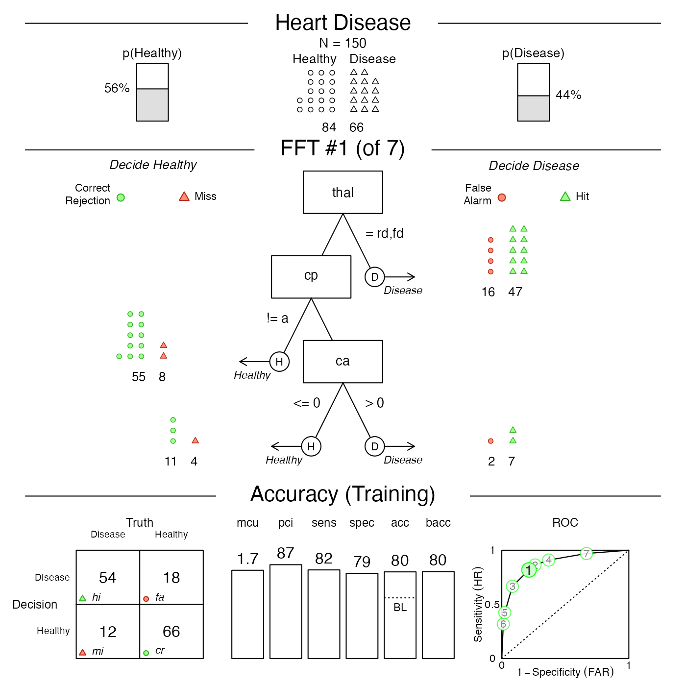
Once we have created an FFTrees object using the FFTrees() function we can visualize the tree (and ROC curves) using the plot() function. The following code will visualize the best training tree applied to the test data:

plot(heart.fft,
     main = "Heart Disease",
     decision.labels = c("Healthy", "Disease"))

See the Plotting FFTrees objects vignette for more details on visualizing trees.

Manually defining an FFT

We can also design a specific FFT and apply it to a dataset by using the my.tree argument of FFTrees(). To do so, we specify the FFT as a sentence, making sure to correctly spell the cue names as they appear in the data. Sets of factor cues can be specified using (curly) brackets.

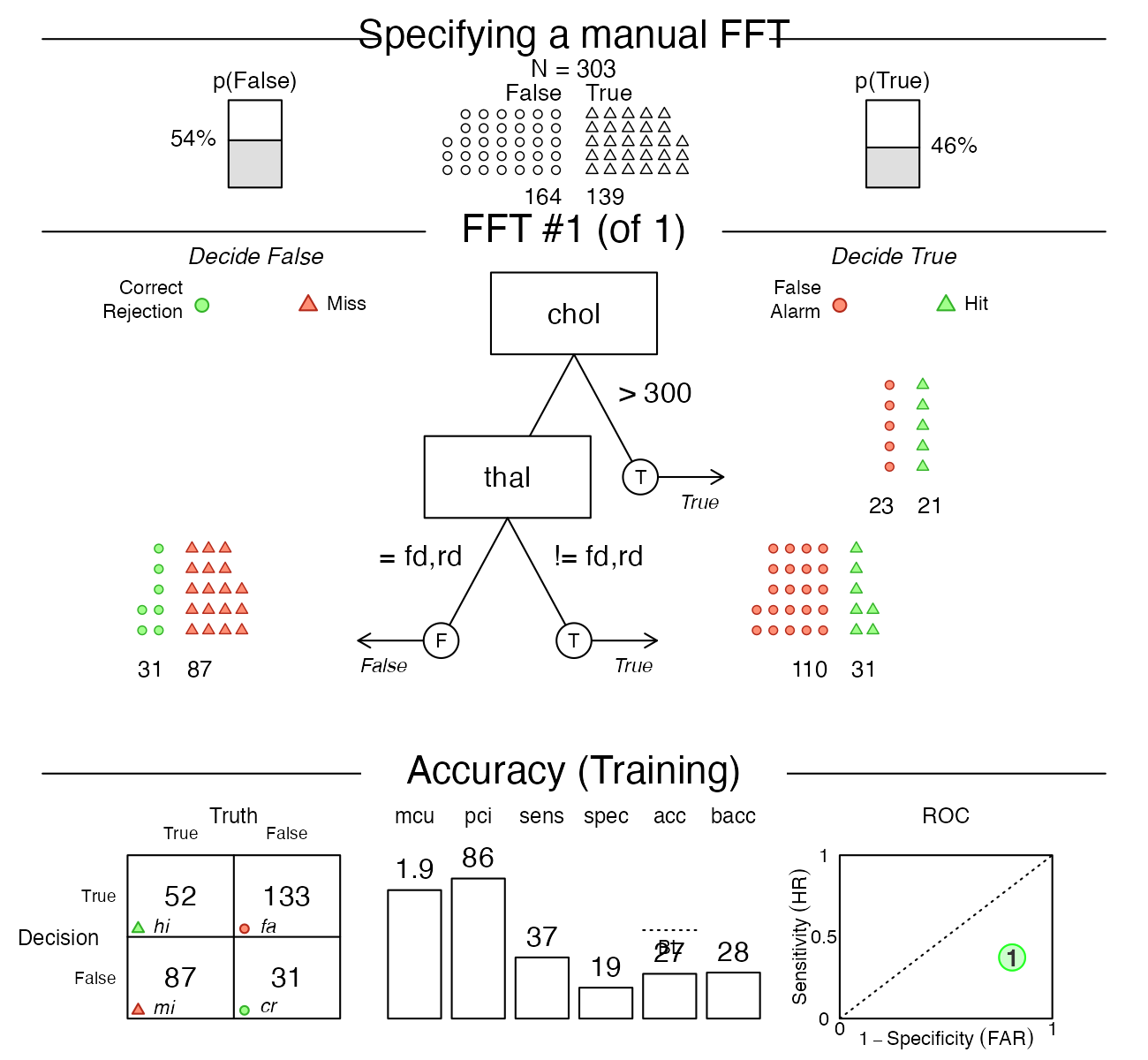
For example, we can manually define an FFT by using the sentence:

"If chol > 300, predict True. If thal = {fd,rd}, predict False. Otherwise, predict True"

# Manually define a tree using the my.tree argument:
myheart_fft <- FFTrees(diagnosis ~., 
                       data = heartdisease, 
                       my.tree = "If chol > 300, predict True. 
                                  If thal = {fd,rd}, predict False. 
                                  Otherwise, predict True")

Here is a plot of the resulting FFT:

plot(myheart_fft, 
     main = "Specifying a manual FFT")

As we can see, the performance of this particular tree is pretty terrible — but this should motivate you to build better FFTs yourself!

In addition to defining an FFT from its verbal description, we can edit and define sets of FFT definitions and evaluate them on data. See the Manually specifying FFTs vignette for details on editing, modifying, and evaluating specific FFTs.

Vignettes

Here is a complete list of the vignettes available in the FFTrees package:

	Vignette	Description
	Main guide: FFTrees overview	An overview of the FFTrees package
1	Tutorial: FFTs for heart disease	An example of using `FFTrees()` to model heart disease diagnosis
2	Accuracy statistics	Definitions of accuracy statistics used throughout the package
3	Creating FFTs with FFTrees()	Details on the main `FFTrees()` function
4	Manually specifying FFTs	How to directly create FFTs without using the built-in algorithms
5	Visualizing FFTs	Plotting `FFTrees` objects, from full trees to icon arrays
6	Examples of FFTs	Examples of FFTs from different datasets contained in the package

References

Phillips, N. D., Neth, H., Woike, J. K., & Gaissmaier, W. (2017). FFTrees: A toolbox to create, visualize, and evaluate fast-and-frugal decision trees. Judgment and Decision Making, 12(4), 344–368. https://doi.org/10.1017/S1930297500006239

Nathaniel Phillips and Hansjörg Neth

2024-05-10

Details on the `FFTrees()` function

Example: Predicting heart disease

Creating trees with `FFTrees()`

Elements of an `FFTrees` object

Basic performance characteristics of FFTs

Cue performance information

Tree definitions

Accuracy statistics of FFTs

Classification decisions

Predicting new cases with `predict()`

Visualising trees

Manually defining an FFT

Vignettes

References

Creating FFTs with FFTrees()

Nathaniel Phillips and Hansjörg Neth

2024-05-10

Details on the FFTrees() function

Example: Predicting heart disease

Creating trees with FFTrees()

Elements of an FFTrees object

Basic performance characteristics of FFTs

Cue performance information

Tree definitions

Accuracy statistics of FFTs

Classification decisions

Predicting new cases with predict()

Visualising trees

Manually defining an FFT

Vignettes

References

Details on the `FFTrees()` function

Creating trees with `FFTrees()`

Elements of an `FFTrees` object

Predicting new cases with `predict()`