Accuracy statistics in FFTrees
Nathaniel Phillips and Hansjörg Neth
2026-04-30
Source:vignettes/FFTrees_accuracy_statistics.Rmd
FFTrees_accuracy_statistics.RmdAccuracy Statistics in FFTrees
In this vignette, we cover how accuracy statistics are calculated for FFTs and the FFTrees package (as described in Phillips et al., 2017). Most of these measures are not specific to FFTs and can be used for any classification algorithm.
First, let’s examine the accuracy statistics from an FFT predicting heart disease:
# Create an FFTrees object predicting heart disease:
heart.fft <- FFTrees(formula = diagnosis ~.,
                     data = heartdisease)
Running this FFTrees() function call yields a new
FFTrees object heart.fft. Both printing or
plotting this object for a particular dataset and tree yields
corresponding accuracy and frugality statistics. For now, we simply plot
the best training tree:
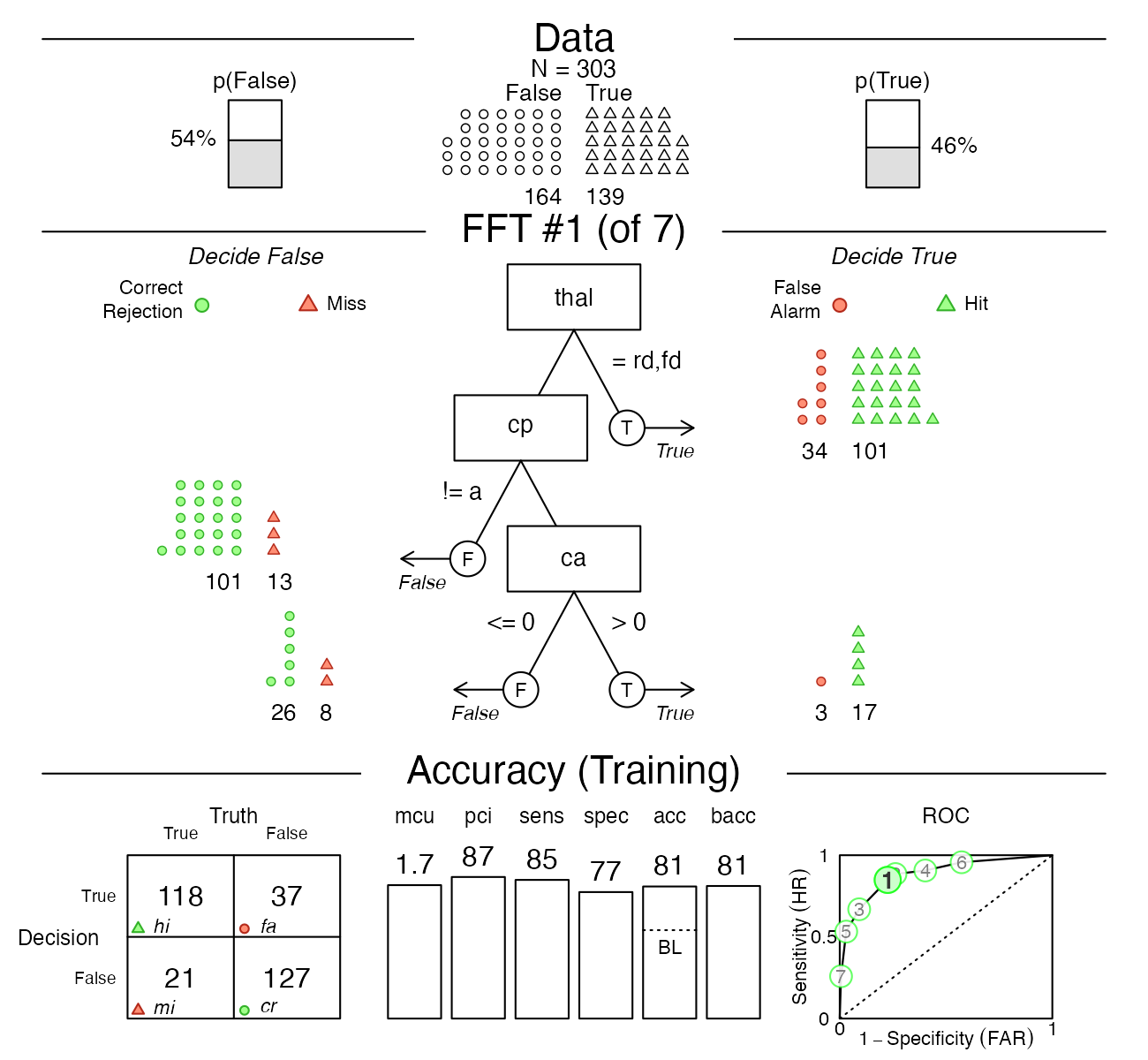
plot(heart.fft, tree = "best.train")
Figure 1: Example FFT for the heartdisease
data.
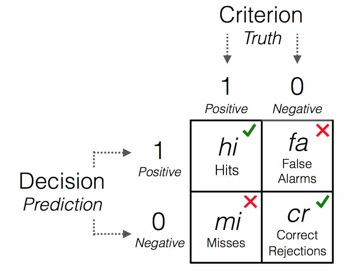
We notice a 2x2 table in the bottom-left corner of the plot: This is a 2 x 2 matrix or confusion table (see Wikipedia or Neth et al., 2021 for details). A wide range of accuracy measures can be derived from this seemingly simple matrix. Here is a generic version of a confusion table:

Figure 2: A 2x2 matrix illustrating the frequency counts of 4 possible outcomes.
A 2 x 2 matrix cross-tabulates the decisions of the algorithm (rows) with actual criterion values (columns) and contains counts of observations for all four resulting cells. Counts in cells a and d refer to correct decisions due to a match between predicted and criterion values, whereas counts in cells b and c refer to errors due to the mismatch between predicted and criterion values. Both correct decisions and errors come in two types:
Correct decisions in cell hi represent hits, positive criterion values correctly predicted to be positive, and cell cr represents correct rejections, negative criterion values correctly predicted to be negative.
As for errors, cell fa represents false alarms, negative criterion values erroneously predicted to be positive, and cell mi represents misses, positive criterion values erroneously predicted to be negative.
Given this structure, an accurate decision algorithm aims to maximize the frequencies in cells hi and cr while minimizing those in cells fa and mi.
| Output | Description | Formula |
|---|---|---|
hi |
Number of hits | |
mi |
Number of misses | |
fa |
Number of false-alarms | |
cr |
Number of correct rejections | |
N |
Total number of cases |
Table 1: Definitions of the frequency counts in a 2x2 confusion table. The notation means number of cases (or frequency counts).
Conditional accuracy statistics
The first set of accuracy statistics are based on subsets of the data. These subsets result from focusing on particular cases of interest and computing conditional probabilities based on them. Given the 2x2 structure of the confusion table, measures can be conditional on either algorithm decisions (positive predictive vs. negative predictive values) or criterion values (sensitivity vs. specificity). In other words, these measures are conditional probabilities that are based on either the rows or columns of the confusion table:
| Output | Description | Formula |
|---|---|---|
sens |
Sensitivity | |
spec |
Specificity | |
far |
False alarm rate |
(spec) |
ppv |
Positive predictive value | |
npv |
Negative predictive value |
Table 2: Conditional accuracy statistics based on either the rows or columns of a 2x2 confusion table.
The sensitivity (aka. hit-rate) is defined as and represents the percentage of cases with positive criterion values that were correctly predicted by the algorithm. Similarly, specificity (aka. correct rejection rate, or the complement of the false alarm rate) is defined as and represents the percentage of cases with negative criterion values correctly predicted by the algorithm.
The positive-predictive value and negative predictive value are the flip-sides of and , as they are conditional accuracies based on decision outcomes (rather than on true criterion values).
Aggregate accuracy statistics
Additional accuracy statistics are based on all four cells in the confusion table:
| Output | Description | Formula |
|---|---|---|
acc |
Accuracy | |
bacc |
Balanced accuracy | |
wacc |
Weighted accuracy | |
bpv |
Balanced predictive value | |
dprime |
D-prime |
Table 3: Aggregate accuracy statistics based on all four cells of a 2x2 confusion table.
Overall accuracy (acc) is defined as the
overall percentage of correct decisions ignoring the difference between
hits and correct rejections. The more specific
measures
and
are averages of sensitivity and specificity,
while
is an average of predictive values. The
measure is the difference in standardized
(-score)
transformed
and (see Luan et al., 2011 for the relation between
FFTs and signal detection theory, SDT).
Speed and frugality statistics
The next two statistics measure the speed and frugality of a fast-and-frugal tree (FFT). Unlike the accuracy statistics above, they are not based on the confusion table. Rather, they depend on how much information FFTs use to make their predictions or decisions.
| Output | Description | Formula |
|---|---|---|
mcu |
Mean cues used: Average number of cue values used in making classifications, averaged across all cases | |
pci |
Percentage of cues ignored: Percentage of cues ignored when classifying cases |
Table 4: Measures to quantify the speed and frugality of FFTs.
To see exactly where these statistics come from, let’s look at the
results for heart.fft (Tree #1):
heart.fft#> FFTrees
#> - Trees: 7 fast-and-frugal trees predicting diagnosis
#> - Cost of outcomes: hi = 0, fa = 1, mi = 1, cr = 0
#> - Cost of cues:
#> age sex cp trestbps chol fbs restecg thalach
#> 1 1 1 1 1 1 1 1
#> exang oldpeak slope ca thal
#> 1 1 1 1 1
#>
#> FFT #1: Definition
#> [1] If thal = {rd,fd}, decide True.
#> [2] If cp != {a}, decide False.
#> [3] If ca > 0, decide True, otherwise, decide False.
#>
#> FFT #1: Training Accuracy
#> Training data: N = 303, Pos (+) = 139 (46%)
#>
#> | | True + | True - | Totals:
#> |----------|--------|--------|
#> | Decide + | hi 118 | fa 37 | 155
#> | Decide - | mi 21 | cr 127 | 148
#> |----------|--------|--------|
#> Totals: 139 164 N = 303
#>
#> acc = 80.9% ppv = 76.1% npv = 85.8%
#> bacc = 81.2% sens = 84.9% spec = 77.4%
#>
#> FFT #1: Training Speed, Frugality, and Cost
#> mcu = 1.73, pci = 0.87
#> cost_dec = 0.191, cost_cue = 1.733, cost = 1.924According to this output, Tree #1 has mcu = 1.73 and
pci = 0.87. We can easily calculate these measures directly
from the x$levelout output of an FFTrees
object. This object contains the tree level (i.e., node) at which each
case was classified:
# A vector of levels/nodes at which each case was classified:
heart.fft$trees$decisions$train$tree_1$levelout
#> [1] 1 3 1 2 2 2 3 3 1 1 1 2 1 1 1 2 1 3 2 2 2 2 2 1 1 2 2 2 3 1 2 1 2 1 2 3 1
#> [38] 1 1 2 1 1 2 2 3 1 2 1 2 2 2 1 3 2 1 1 1 1 2 2 1 2 1 2 1 1 2 1 1 2 2 1 1 1
#> [75] 3 2 1 2 2 1 3 3 2 1 2 2 2 2 3 2 3 1 1 2 2 1 1 1 2 3 3 2 3 2 1 1 1 1 1 1 1
#> [112] 3 1 1 1 1 2 3 1 1 1 1 2 1 2 2 1 1 2 3 1 1 2 3 2 2 1 1 1 2 2 1 2 1 1 2 1 2
#> [149] 2 2 1 3 1 1 3 3 1 1 1 1 1 3 2 3 2 1 2 2 1 2 1 1 3 3 1 1 1 1 2 2 1 1 2 1 3
#> [186] 2 1 1 1 1 2 1 1 3 2 3 2 3 2 2 3 3 1 1 1 1 1 1 2 3 2 1 2 1 3 1 2 3 3 3 2 2
#> [223] 2 1 3 2 3 2 3 3 2 3 2 2 2 3 1 1 2 2 2 2 3 2 2 3 1 3 1 2 1 1 1 2 3 2 3 2 2
#> [260] 1 2 2 2 2 3 1 3 1 1 2 1 1 1 3 2 1 2 2 2 3 1 2 1 2 1 1 1 1 1 2 1 2 1 1 3 2
#> [297] 1 1 1 1 1 2 2Now, to calculate mcu (the mean number of cues
used), we simply take the mean of this vector:
# Calculate the mean number or cues used (mcu):
mean(heart.fft$trees$decisions$train$tree_1$levelout)
#> [1] 1.732673Now that we know where mcu comes from, computing
pci (i.e., the percentage of cues ignored) is just
as simple — it’s just the total number of cues in the dataset
minus mcu, divided by the total number of cues in the
data:
# Calculate pci (percentage of cues ignored) as
# (n.cues - mcu) / n.cues):
n.cues <- ncol(heartdisease)
(n.cues - heart.fft$trees$stats$train$mcu[1]) / n.cues
#> [1] 0.8762376Additional measures
There is a wide range of additional measures that can be used to
quantify classification performance. Most of these can easily be
computed from the numerical information provided in an
FFTrees object. For alternative measures based on the
frequency counts of a 2x2 matrix, see Table
3 of Neth et al. (2021).
Vignettes
Here is a complete list of the vignettes available in the FFTrees package:
| Vignette | Description | |
|---|---|---|
| Main guide: FFTrees overview | An overview of the FFTrees package | |
| 1 | Tutorial: FFTs for heart disease | An example of using FFTrees() to model
heart disease diagnosis |
| 2 | Accuracy statistics | Definitions of accuracy statistics used throughout the package |
| 3 | Creating FFTs with FFTrees() | Details on the main FFTrees()
function |
| 4 | Specifying FFTs directly | How to directly create FFTs without using the built-in algorithms |
| 5 | Visualizing FFTs | Plotting FFTrees objects, from full trees
to icon arrays |
| 6 | Examples of FFTs | Examples of FFTs from different datasets contained in the package |