Text boxes and decorations

This vignette explains the unikn functions for plotting graphical elements and text decorations. (See the vignette on colors for general information on colors, color palettes, and corresponding functions, or the more specialized vignettes on color recipes and institutional colors.)

Please install and/or load the unikn package to get started:

# install.packages('unikn')  # install unikn from CRAN client
library('unikn')             # loads the package

Overview

Beyond providing support for colors, unikn provides functions for plotting graphical elements (like boxes) and text decorations (with colored backgrounds or underlining). Before illustrating these functions, please note some caveats:

Plotting text (i.e., graphically rendering characters) is rarely a good idea. In contrast to the vector fonts used by DTP programs, plotted text typically does not scale (when changing the size of images) and cannot be recognized automatically (e.g., copied, indexed, or scraped). Hence, the following functions should only be used when no better solutions are available (e.g., for adding text to graphs, or for obstructing automatic text recognition).
Like all other templates, our renderings are subject to constraints and limitations. For instance, as any standard installation of R lacks the prescribed “Theinhardt” fonts, we only mimic the official design specifications (in Arial, sans serif).

That said, digital decorations can be useful to emphasize or structure information, provided that they can be produced easily and flexibly. The unikn package helps preventing common mistakes by novices (e.g., boxes or lines extending beyond text, or step-functions in multi-line headings) and can be customized and improved by expert users. Hence, we hope that the following functions are useful for plotting graphical elements (e.g., boxes, logos, etc.) and help you achieve a uniform look when styling presentations or visualizations.

Please load the unikn package to get started:

library(unikn)  # load unikn package

Plotting empty slides and boxes

As the text functions of unikn add styled text to an existing plot, we must first create a plot to which we can add text. unikn provides 2 basic functions for creating new plots:

slide plots an empty canvass (a rectangular box or frame);
xbox plots a colored box with an X in its top right corner.

Here are both commands with their default settings:

slide()  # plot default slide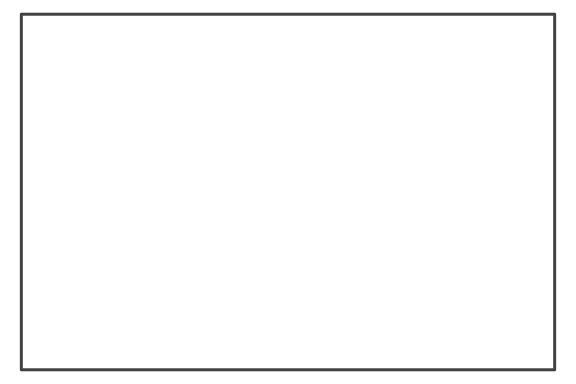

xbox()  # plot default xbox

Both functions accept additional arguments to customize their appearance.

Colors

The background and border colors of slides can be changed by setting their col, border, and lwd arguments:

slide(col = pal_seeblau[[1]], border = Petrol, lwd = 5)  # set colors of slide background and border

slide(col = pal_peach[[2]], border = NA)  # colored slide without a border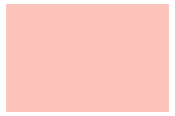

Similarly, the background color of xboxes can be changed by the col argument:

xbox(col = Pinky)  # set background color of xbox

Dimensions

By default, both slide and xbox fill the entire plotting region (i.e., all margins are set to 0).

The width of a slide is set to 4/3 of its height (of 1). To change this default, use the dim argument for specifying the slide’s x- and y-dimensions, respectively:

slide(dim = c(3, 1))  # a slide 3x wider than high

Note that changes in slide dimensions are invisible when viewing images interactively, as R automatically scales images to the size of the canvass. They mostly affect the relation between metrics when adding elements to an object.

Similarly, an xbox has the default dimensions of a unit square (i.e., dim = c(1, 1)). To change this default, use the dim argument for specifying the xbox’s x- and y-dimensions, respectively:

xbox(col = Petrol, dim  = c(1, 2))  # an xbox 2 times higher than wide

The two strokes of the X (in the top right corner) are orthogonal when viewing the xbox at the aspect ratio indicated by dim (i.e., here: at a ratio of width x = 1 to height y = 2). When viewing the box at any different aspect ratio, the X appears to be distorted. Hence, viewing and printing plots at the desired aspect ratio helps when creating an xbox.

Plotting styled text

There are three main functions for plotting text with decorations:

mark() allows highlighting text with colored background boxes;
uline() allows underlining text with colored lines;
post() allows posting text in rectangular xbox elements.

In addition, there are 2 auxiliary functions:

headline() allows plotting headlines with colored background boxes;
url_unikn() allows formatting URLs the uni.kn way.

The following sections illustrate the functions and their main options in turn.

Mark text

The mark() function allows highlighting text by plotting it with colored background boxes (to provide the functionality of “Markieren”):

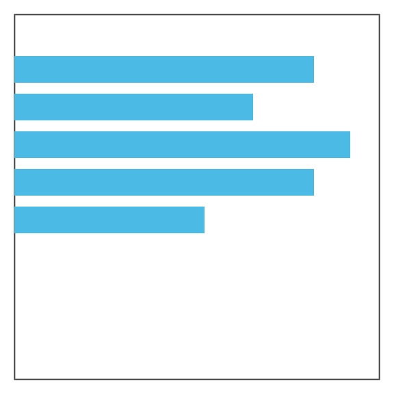
By default, mark() assumes that we want to add highlighted text to an existing plot. The text labels to be added are provided (as a character vector) by the labels argument, their coordinates as the corresponding x and y arguments. Various text decorations (i.e., text and background colors, text sizes, and font types) can be set by specifying additional arguments (i.e., col, col_bg, cex, and font, respectively):

# Some pre-existing plot: 
n <- 20
set.seed(1)
par(mar = c(0, 0, 0, 0))
plot(x = runif(n), y = runif(n), type = "p", pch = 16, cex = 20, col = grey(0, .2),
     axes = FALSE, xlab = "", ylab = "")

# Add 1 marked label:
mark(labels = "Some messy plot", x = .02, y = .9)

# Add 2 more marked labels:
mark(labels = c("Note something here.", "More highlighting here."), 
     x = c(.1, .6), y = c(.2, .4),
     col_bg = c(pal_seeblau[[2]], pal_peach[[3]]), cex = 1.2)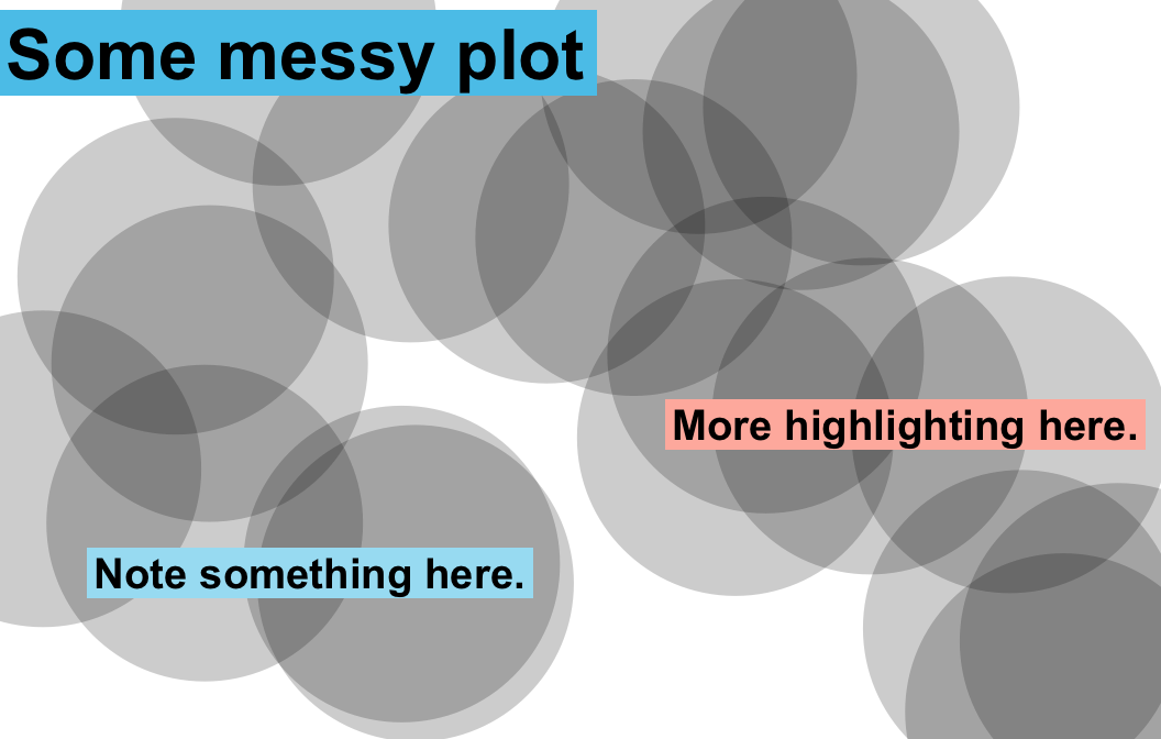

If no pre-existing plot is available, setting the new_plot argument to either "blank" or "slide" will generate a new default plot (by calling the slide() function described above):

# A sentence to plot: 
s <- c("Markieren",
       "ist ein Bestandteil",
       "von Studieren.")

# Create a new plot (of type "slide"):
mark(labels = s,
     x = 0, y = .85, y_layout = .03,
     col_bg = Seeblau,
     cex = 1.5,
     new_plot = "slide")

# Add text to the same plot:
mark(labels = s,
     x = 0, y = .40, y_layout = .03,
     col_bg = pal_pinky[[2]],
     cex = 1.5, 
     new_plot = "none")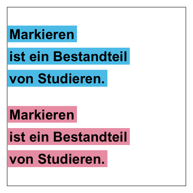

Rather than providing explicit x and y coordinates for all text elements in labels, the calls above defined an initial coordinate and used a numeric y_layout argument to fix the distance between consecutive text labels (to a value of .03).

As an alternative to numeric coordinates and position values, x_layout and y_layout also accept some special values (as character strings):

x_layout accepts:
- x_layout = "center" for centering labels horizontally (on the first label or the middle),
- x_layout = "left" left-justifies labels (on the first label or the middle), and
- x_layout = "right" right-justifies labels (on the first label or the middle).
y_layout accepts:
- y_layout = "even" for an even distribution of labels across the available y-space, and
- y_layout = "flush" to omit space between adjacent labels (as in y_layout = 0).

Thus, the position and orientation of the text labels can be controlled by using the x_layout and y_layout options:

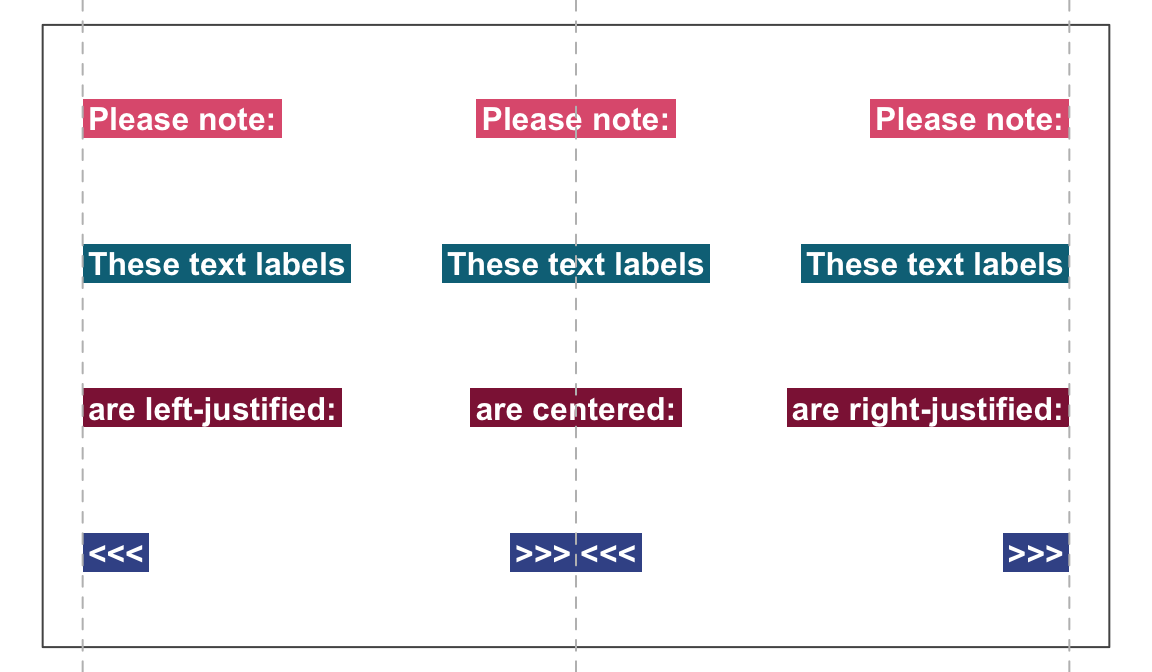
See ?mark for details.

Underline text

The uline() function allows emphasizing text by plotting it with colored underlining (to provide the functionality of “Unterstreichen”):

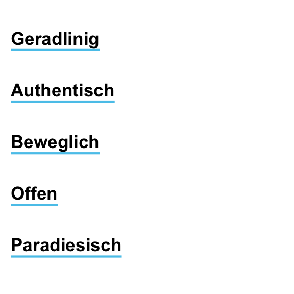
As with mark() above, the uline() command distinguishes between creating a new plot (by setting new_plot to either "blank" or “slide”) or adding to a pre-existing plot (by using the default new_plot = "none"):

lbl_uline <- c("This is neat, true, and terribly important")
uline(labels = lbl_uline, new_plot = "blank", y = .6, cex = 1.1)  # create a new plot
uline(labels = "(which is why we underline it).", y = .45, cex = 1)  # add to plot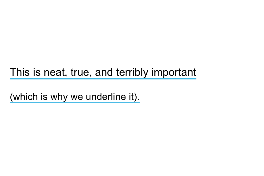

The arguments for text elements (labels), text positions (x, y, y_layout), and text properties and decorations (col, col_bg, cex, and font) work as they do for mark(). For instance, shorter vectors are recycled to match the length of labels:

slogan <- c("Geradlinig", "Farbenfroh", "Beweglich", "Bunt", "Paradiesisch")
uline(labels = slogan,
      x = c(0, .5), y = .9, y_layout = "even",
      col = c("black", Bordeaux), col_bg = c(Seeblau, Seegruen), 
      cex = 1.1, font = 2, new_plot = "blank")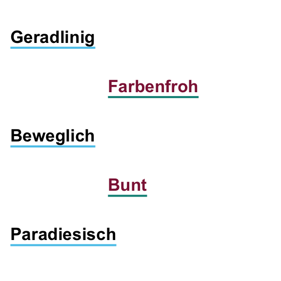

The position and orientation of the text labels can be controlled by using the x_layout and y_layout options:

Post text

The post() function allows adding text to a rectangular xbox (to provide the functionality of “Merken”):

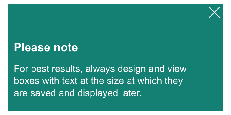
By default, post() assumes a pre-existing xbox to which the text elements of labels are to be added.
For square boxes, setting new_plot to "xbox" creates a new xbox with its default dimensions of dim = c(1, 1).
By adjusting its color and text arguments, post() allows creating simple badges or logos:

# Badge (to view as 250 x 250 pixel):
post(labels = "ToDo", y = .35, 
     col = "white", col_bg = pal_signal[[1]],
     cex = 3, font = 2, new_plot = "xbox")  

# Badge (to view as 250 x 250 pixel):
post(labels = "R", y = .35, 
     col = "white", col_bg = pal_seeblau[[5]],
     cex = 8, font = 2, new_plot = "xbox")

Another potential use of post() is for creating images providing contact details:

address <- c("Dr. B. F. Skinner", " ",
             "Department of Psychology",
             "Office Z101",
             "Tel.: +49 7531 88-0815",
             "Fax: +49 7531 88-0810",
             "b.f.skin@uni-konstanz.de")

post(labels = "Contact",
     y = .7,
     cex = 1.2, font = 2,
     col_bg = Petrol,
     new_plot = "xbox")  # create new plot 

post(labels = address,
     y = .5, y_layout = .03,
     new_plot = "none")  # add to plot

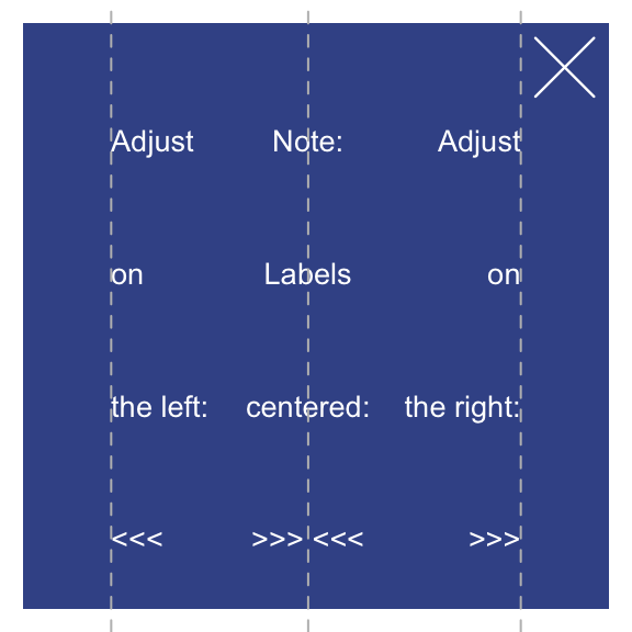
As above, the position and orientation of the text labels can be controlled by using the x_layout and y_layout options:

Headings

The heading() function makes it easy to create recognizable headings:

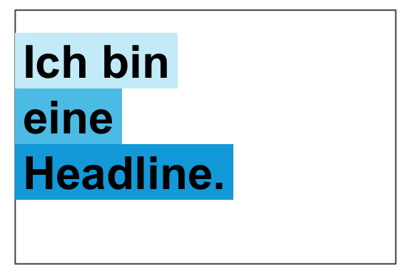
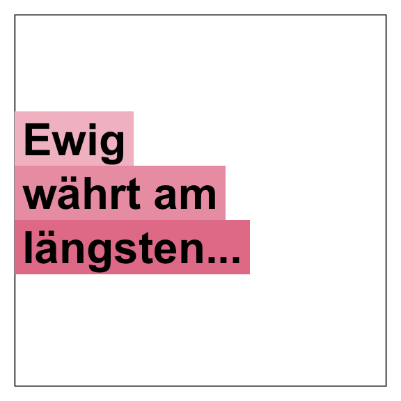
By default, the function creates a new slide (i.e., new_plot = "slide") and positions the text elements of labels on its left edge (i.e., x = 0, y = .8 and y_layout = "flush"). When headings violate the official recommendations, a message is provided:

heading(labels = c("Ewig", "währt am", "längsten..."), 
        y = 2/3, col_bg = usecol(pal_pinky))

Re-arranging words helps to avoid step-wise titles (see p. 25 of the CD manual):

# Beware of step-wise arrangements:
heading(labels = c("Ich", "bin keine", "gute Headline."))
#> Step-wise titles are discouraged: Consider re-arranging?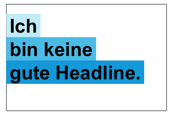


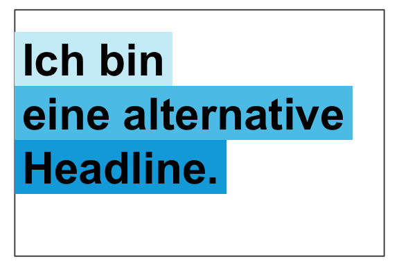
# Avoiding warning:
heading(labels = c("Ich bin", "eine alternative", "Headline."))

When colors are left unspecified, heading() selects colors that are appropriate for the number of elements in labels (i.e., shades of Seeblau for col_bg = "default"). However, default colors can be overwritten by setting the col and col_bg arguments:

heading(labels = c("Ene,", "mene, miste,", "es rappelt", "in der Kiste."), 
        col = "white", col_bg = c(Pinky, Seegruen, Bordeaux, Karpfenblau))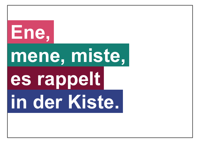

URLs

One of the more obscure rules (on p. 31 of the CD manual) concerns the rendering of URLs, in which typical web patterns (like “http” or “www”) are to be omitted and replaced by a typographical dash (which is longer than a hyphen). The url_unikn utility function allows formatting URLs the uni.kn way:

my_url <- url_unikn("https://www.uni-konstanz.de/")  # input URL
my_url # formatted URL
#> [1] "– uni-konstanz.de"

# Put URL at bottom of an xbox:
post(labels = my_url, x = .05, y = .1, font = 4, 
     col_bg = pal_seeblau[[5]], new_plot = "xbox")

Resources

The following versions of unikn and corresponding resources are currently available:

Type:	Version:	URL:
A. unikn (R package):	Release version	https://CRAN.R-project.org/package=unikn
	Development version	https://github.com/hneth/unikn/
B. Online documentation:	Release version	https://hneth.github.io/unikn/
	Development version	https://hneth.github.io/unikn/dev/

Vignettes

The following vignettes provide instructions and examples for using the unikn colors, color palettes, and functions:

Nr.	Vignette	Content
1.	Colors	Colors and color functions
2.	Color recipes	Recipes for color-related tasks
3.	Institutional colors	Creating color palettes for other institutions
4.	Text	Text boxes and decorations

SPDS, uni.kn

2023 01 01