Institutional colors

The color palettes included in the unikn package are based on the CD manual of the University of Konstanz. However, the functionality provided by the package makes it easy and straightforward to define and use your own colors.

Version 0.8.0 of unikn (released in 2023-01-06) contained 52 additional color palettes from other institutions (mostly universities).

As the number of color palettes has been growing beyond the scope of this package, the color palettes from other institutions are now being collected in a separate R package unicol.

Installing unicol currently provides access to a diverse range of over 200 color palettes from over 80 institutions.

The rest of this vignette explains how the color-related tools of unikn can be used for creating new color palettes. If you do so, please consider submitting it to be included in future versions of the unicol package. (For a general introduction of the unikn colors, color palettes, and color functions, see the vignettes on Colors and color functions and Color recipes. The vignette on Text boxes and decorations provides information on plotting slides and text elements.)

We install or load the unikn package to get started:

# install.packages('unikn')  # install unikn from CRAN client
library('unikn')             # load the package

Creating new color palettes

A color palette is an ordered collection of color objects. Creating new color palettes in R is simple and only requires two steps:

Define the palette’s elementary colors as R objects.
Combine colors into a color palette.

In the following, we illustrate both steps. As we will see, Step 1 can either be omitted (when the to-be-combined colors exist as R objects) or can be included in Step 2.

As an example, we will re-create the color palette of the German Max Planck Society (that unikn exports as mpg_pal) from the color definitions in its Corporate Design manual (available here).

1. Defining colors

Before we can a create new color palette in R, its elementary colors need to exist as R objects. (If all colors to-be-combined into a new palette exist as R objects, we can skip this step and directly proceed to 2. Combining colors into a palette.) Defining new colors in R requires a basic understanding of their underlying representation.

How colors are represented and perceived is a wide-ranging topic that has fascinated scholars and practitioners for centuries. Essentially, there are many alternative ways to analyze or synthesize colors, and the most appropriate representational way depends on the specific context of a particular use case (see Wikipedia: Color model for an introduction).

In R, the grDevices package (included in any default installation) provides colors and color-related functions. Although R supports many color models (including HCL, HSV, Lab, Luv, and RGB variants), the three most common ways of expressing colors in R are:

by R color name: R includes 657 named colors, whose names are provided (as a character vector) by evaluating the colors() function of grDevices.
by RGB values: Every color (or hue) is expressed by a triple of numeric values on three dimensions that denote the additive primary colors (red, green, blue). The range of values is either expressed on a scale from 0 to 1, or — more typically — on a scale from 0 to 255 (i.e., on an 8 bit scale allowing for \(2^8 = 256\) different values).
by HEX values: Every color (or hue) is expressed by a character string (with the prefix #), followed by a triple of hexadecimal values (each ranging from 00 to FF) that correspond to the triple of decimal RGB values (in the range from 0 to 255).

Importantly, the same color (or hue) can be denoted by its name, its RGB values, and its HEX values. Thus, the three different systems (i.e., color name, RGB values, or HEX values) can be alternative representations of the same object. However, just as the properties of an alphabet or numeral notation system constraints the words or numbers that can be expressed by it, the universe of possible colors is limited by their representation. For instance, whereas the RGB and HEX systems usually distinguish between more than 16 million (i.e., \((2^8)^3 = 256^3 = 16.777.216\)) possible colors, only a limited number of them are named. Similarly, when multiple names refer to the same triple of RGB or HEX values, they denote the same color.¹

An example helps clarifying these abstract terms. When viewing an existing color or color palette with the seecol() function of unikn, the name, HEX and RGB values of the individual colors are being shown. For instance, the following color palette mpg_pal provides the colors of the Max Planck Society:

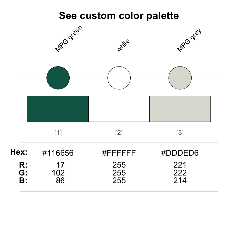
As the middle color of mpg_pal is one of the 657 named colors of colors(), R will recognize it as a color when we type its name (as a character object "white") in a context that expects color inputs. However, the two other colors of mpg_pal have specifically been defined by the Max Planck Society and thus are not pre-defined colors of R (i.e., not contained in colors()). To use such colors in R, we first need to define them as color objects.

So how can we define new colors in R? Most institutions will provide definitions of their corporate colors or instructions how they can be defined in some standard color system. Unfortunately, some definitions (such as those using the subtractive CMYK model) are aimed at printing (as opposed to computer screens) and other standards (such as numeric PANTONE™ PMS codes) are proprietary. But as most institutions have an interest in widely disseminating their colors, they typically include translations or approximations for alternative color models in their definitions.

The Max Planck Society defines two main colors in its CD manual (available here):

A dark shade of green is defined as Pantone 328, and approximated by CMYK 100/0/57/30 or RGB 17/102/86.
A light shade of grey is Pantone 427, and approximated by CMYK 0/0/6/15 or RGB 221/222/214.

In the following, we will first use the RGB values to define both colors (as these are provided in the definition). However, we then show that we alternatively could have used the colors’ HEX values (had they been provided) to define the same color objects.

Defining colors from their RGB values

As our two colors of interest are given in RGB values, we can use the rgb() function of the grDevices package to define corresponding objects:

mpg_green <- grDevices::rgb( 17, 102,  86, maxColorValue = 255)
mpg_grey  <- grDevices::rgb(221, 222, 214, maxColorValue = 255)

The first three arguments specify values on the red, green, and blue dimension, respectively. Importantly, the values must be in the range \([0, max]\), where \(max\) is provided by maxColorValue = 255. Whereas the sRGB standard expresses all values in a normalized range of \([0, 1]\), most color definitions use the traditional 8-bit representation that distinguish between \(2^8 = 256\) levels in the range \([0, 255]\). The rgb() function additionally allows for adding names and a transparency level alpha, but as we can modify these aspects later, we do not need to use them at this point.

What do we obtain when we evaluate our new color objects? Let’s see:

mpg_green
#> [1] "#116656"
mpg_grey
#> [1] "#DDDED6"

When evaluating an object created by rgb(), R returns a character sequence of the form "#rrggbb". In this string, the sequence rrggbb expresses the three RGB values (for the red, green, and blue dimension, respectively) in hexadecimal (HEX) notation (in the range \([0, 255]\)). In HEX notation, the ten numeral symbols (i.e., the digits from 0 to 9) or the decimal system are extended by the first six letters of the alphabet (i.e., A to F) to turn our familiar base-10 notation into an analogous place-value notation with a base of 16. Thus, the HEX values of "#116656" is merely a more compact way of expressing

red: \(1 \cdot 16 + 1 = 17\)
green: \(6 \cdot 16 + 6 = 102\)
blue: \(5 \cdot 16 + 6 = 86\)

Thus, the HEX values "#116656" provide an alternative way of expressing the RGB values 17/102/86 — and both refer to the color “MPG green” (shown as mpg_pal[1] above).

Defining colors from their HEX values

The equivalence of the RGB and HEX notations can be illustrated by defining the same colors a second time, but this time specifying their HEX values (returned above):

mpg_green_2 <- "#116656"
mpg_grey_2  <- "#DDDED6"

If both definitions really yield identical R objects, the following checks must evaluate to TRUE:

all.equal(mpg_green, mpg_green_2)
#> [1] TRUE
all.equal(mpg_grey,  mpg_grey_2)
#> [1] TRUE

Thus, we can define colors from both their RGB or HEX values — and the two notations are really just two alternative ways of representing the same colors.

2. Combining colors into a palette

Having defined two new colors, we can easily combine them into a new color palette. A color palette is simply a sequence of colors that are stored in some sequential data structure. The two simplest data structures in R that are suited for this purpose are vectors or data frames. Thus, the following two expressions both define valid color palettes:

c(mpg_green, mpg_grey)
#> [1] "#116656" "#DDDED6"
data.frame(mpg_green, mpg_grey)
#>   mpg_green mpg_grey
#> 1   #116656  #DDDED6

As it often is easier to remember and access colors by their names, it usually makes sense to name the elements of a color palette (e.g., by using the name() function).

The newpal() function of unikn provides a convenient wrapper for defining color palettes. Its main argument col uses a vector of color objects that make up the new palette, whereas names and as_df allow specifying color names and switching between returning the new palette as a vector or data base.
Importantly, the color objects of col can be provided as RGB values, as R color names, or as HEX values:

mpg_pal_3 <- newpal(col = c(rgb( 17, 102,  86, maxColorValue = 255), "white", "#DDDED6"),
                    names = c("MPG green", "white", "MPG grey"),
                    as_df = FALSE)

The new color palette mpg_pal_3 contains the three basic colors of mpg_pal (shown above):

seecol(mpg_pal_3, 
       main = "My new color palette", col_brd = "black", lwd_brd = .5)

The 5-color palette provided as mpg_pal includes two intermediate colors (at positions mpg_pal[2] and mpg_pal[4]) that are extrapolated by mixing the two main MPG colors with “white” in a balanced (50:50) fashion. The usecol() function of unikn automatically performs these extrapolations when extending a 3-element color palette (e.g., mpg_pal_3) to n = 5 colors:

my_mpg_pal <- usecol(mpg_pal_3, n = 5)

The resulting color palette my_mpg_pal recreates the colors of the unikn color palette mpg_pal (shown above):

seecol(my_mpg_pal, main = "My new MPG color palette", 
       col_brd = "black", lwd_brd = .5)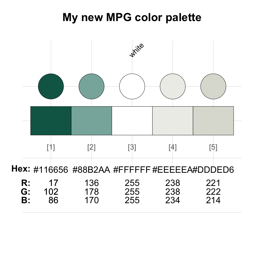

Technically, the two color palettes differ in some names and the way in which its middle color (“white”) was specified (by its R color name or HEX values). However, when using col2rgb() for converting both palettes into their RGB values, we see that they contain the same colors:

all.equal(col2rgb(mpg_pal), col2rgb(my_mpg_pal), check.attributes = FALSE)
#> [1] "Numeric: lengths (9, 15) differ"

This concludes our illustration of defining a new colors and color palettes.

Comparing color palettes

Once a new palette has been defined (and is available in your current R environment), the seecol() and usecol() functions allow comparing, scaling, and using them in the same fashion as the native unikn color palettes:

# Scaled palettes: 
seecol(list(mpg_pal, pal_unikn), n = 7,
       pal_names = c("Max Planck", "Uni Konstanz"),
       main = "Comparing scaled color palettes")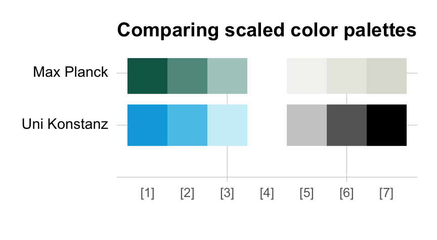

See the vignette on Color recipes for additional examples of using unikn functions for solving color-related tasks.

Call for contributions

We are still expanding the range of color palettes from other institutions in a dedicated R package unicol.

Collecting color palettes

Are you using the unikn color functions to create your own color palettes?

If so, please let us know (e.g., by posting on this GitHub issue)!

We collect color palettes from other institutions to make them available to R users in future versions of unicol.

To enable us to verify and provide credit to your contributions, please send us the following information:

your code (e.g., the newpal() command creating your color palette),
your reference or source information (e.g., some URL with color definitions),
your name and some contact information (e.g., an Email address).

We’re looking forward to your inputs and contributions (at this GitHub issue)!

Resources

The following versions of unikn and corresponding resources are currently available:

Type:	Version:	URL:
A. unikn (R package):	Release version	https://CRAN.R-project.org/package=unikn
	Development version	https://github.com/hneth/unikn/
B. Online documentation:	Release version	https://hneth.github.io/unikn/
	Development version	https://hneth.github.io/unikn/dev/

Vignettes

The following vignettes provide instructions and examples for using the unikn colors, color palettes, and functions:

Nr.	Vignette	Content
1.	Colors	Colors and color functions
2.	Color recipes	Recipes for color-related tasks
3.	Institutional colors	Creating color palettes for other institutions
4.	Text	Text boxes and decorations

Strictly speaking, different shades of a given color can be further distinguished by different opacity or transparency levels (typically denoted by an alpha value). However, the visual appearance of a transparent color can be mimicked by mixing the color with the background color (usually “white”). Hence, transparent shades of a color are usually not counted as different colors.↩︎

SPDS, uni.kn

2023 08 16