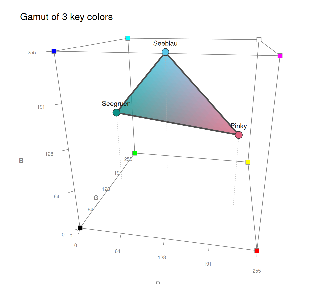
Plot colors as points in a 3D RGB color cube

plot_cube plots one or more colors x as points in a 3-dimensional cube whose axes correspond to the red, green, and blue values of the RGB color model (ranging from 0 to 255).

Usage

plot_cube(
  x,
  type = "p",
  col_points = NA,
  cex_points = 2,
  pch = 21,
  col_brd = grey(0.2, 1),
  ref_lines = TRUE,
  col_line = NA,
  lwd_line = 3,
  line_connect = "all",
  col_fill = NA,
  fill_alpha = 0.8,
  fill_res = 20,
  shadows = "none",
  col_shadow = grey(0.7, 0.9),
  show_corners = TRUE,
  col_cube = grey(0.5, 1),
  grid = FALSE,
  grid_faces = FALSE,
  grid_inner = FALSE,
  grid_at = 2,
  col_grid = grey(0.6, 0.6),
  col_grid_inner = grey(0.8, 0.5),
  axis_labels = c("R", "G", "B"),
  axis_ticks = TRUE,
  n_ticks = 5,
  cex_axis = NA,
  labels = "names",
  theta = -30,
  phi = 15,
  main = "Colors in 3D RGB space",
  cex_lbl = 0.85,
  ...
)

Arguments

x

A (character) vector of colors to be plotted, specified as R color names (e.g., "deepskyblue"), HEX values (e.g., "#59C7EBFF"), or any mixture thereof. Color palettes (e.g., pal_unikn) are also accepted.

type

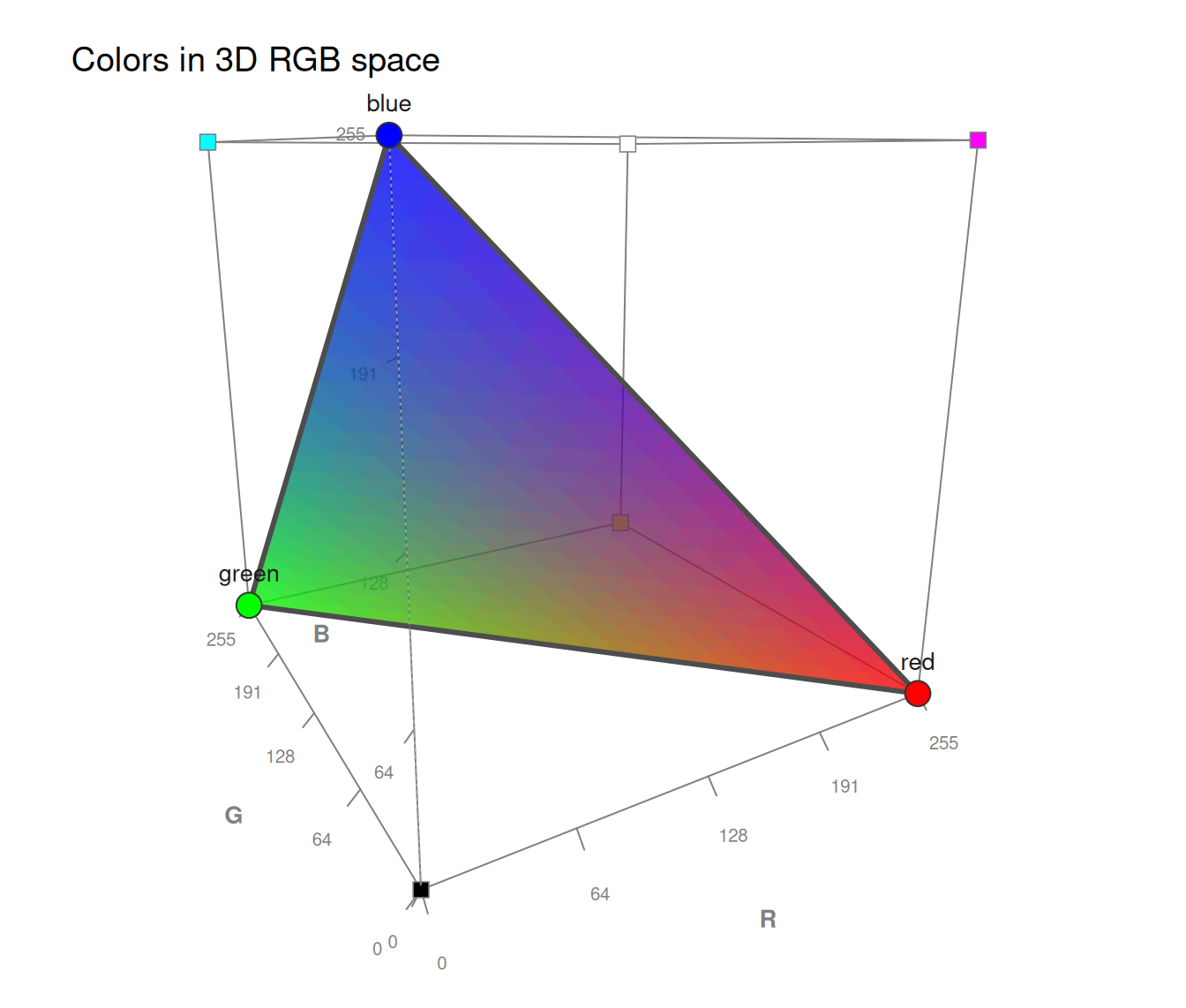
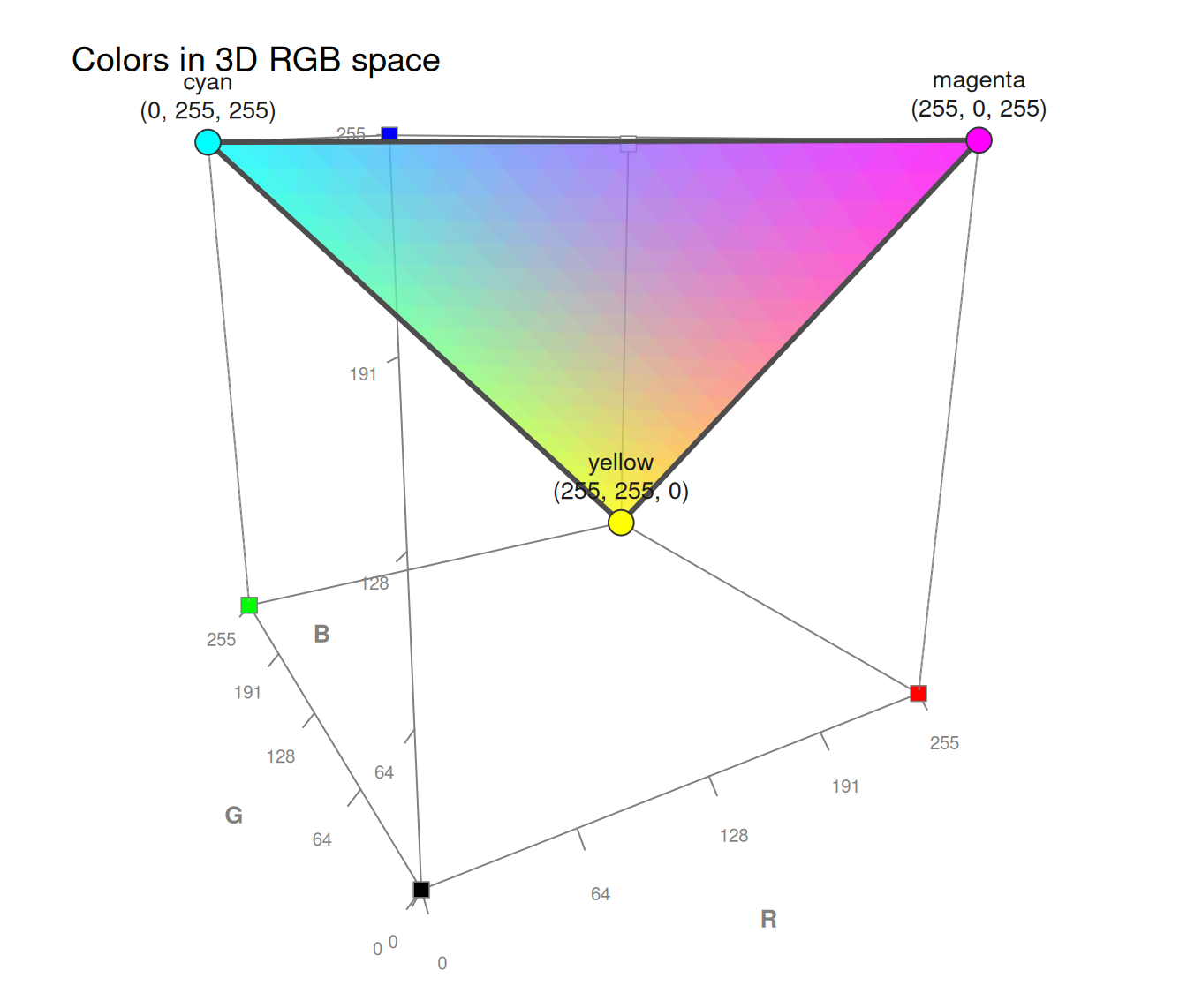
Type of geometric element to draw from the colors x:

"p": Plot colors as points (default);
"l": Connect colors by lines (a path through RGB space);
"b": Draw both points and lines;
"plane": Span a plane (filled polygon) through the colors (requires 3 or more colors; 3 colors yield a triangle).

By default, connecting lines and plane fills are shown as color gradients (i.e., each location is shown in the color of the corresponding RGB mixture), to illustrate the additive mixing of colors in RGB space. In all cases, only the colors x provided (i.e., the points that define the line or plane) are labeled by default (see labels). Default: type = "p".

col_points

Color(s) used for the plotted points. Default: col_points = NA uses each point's own color (i.e., every color in x is plotted in that color). Providing a color (or color vector) overrides this, so that all points are shown in the specified color(s).

cex_points

Scaling factor for the size of points. Default: cex_points = 2.

pch

Plotting symbol for points (see points). Default: pch = 21 (a fillable circle).

col_brd

Border color of points (only used for fillable symbols, i.e., pch in 21:25). Default: col_brd = grey(.20, 1) (dark grey).

ref_lines

Boolean: Draw a vertical reference line from each point down to the base (R-by-G) plane of the cube (to ease judging a point's height on the B/blue axis)? Default: ref_lines = TRUE.

col_line

Color of connecting lines (for type = "l" or "b") and of the plane outline (for type = "plane"). Default: col_line = NA (i.e., show lines as a color gradient of the mixtures between consecutive colors).

lwd_line

Line width of connecting lines (for type = "l" or "b") and of plane outlines (for type = "plane"). Raise this value for thicker, more visible lines. Default: lwd_line = 3.

line_connect

How to connect 3 or more colors by lines (for type = "l" or "b"):

"all": Connect all pairs of colors (i.e., n * (n - 1) / 2 lines, a complete graph);
"pairs": Connect only disjoint consecutive pairs of colors, i.e., (1st, 2nd), (3rd, 4th), etc. (yielding floor(n / 2) lines; if n is odd, the final color remains unpaired, but is still shown as a point);
"path": Connect only consecutive colors (i.e., n - 1 lines, tracing the palette in its given order).

For 2 colors, all 3 options yield the same single line. (The value "pairwise" is accepted as an alias for "all".) Default: line_connect = "all".

col_fill

Fill color for the plane (for type = "plane"). Default: col_fill = NA (i.e., fill the plane with a color gradient showing the gamut of all mixtures of the defining colors).

fill_alpha

Opacity of the plane fill (in range [0, 1]). Default: fill_alpha = .80.

fill_res

Resolution of color gradients (i.e., the number of line segments per connection, and the granularity of the plane tessellation). Higher values yield smoother gradients (but slower plotting). Default: fill_res = 20.

shadows

Project each point onto one or more faces of the cube (as "shadow" points, to aid judging its 3D location). Options (one or more of which may be combined) are:

"floor": project onto the R-by-G plane (i.e., set B = 0);
"back": project onto the R-by-B plane (i.e., set G = 0);
"side": project onto the G-by-B plane (i.e., set R = 0);
"all": project onto all 3 faces;
"none": show no shadows.

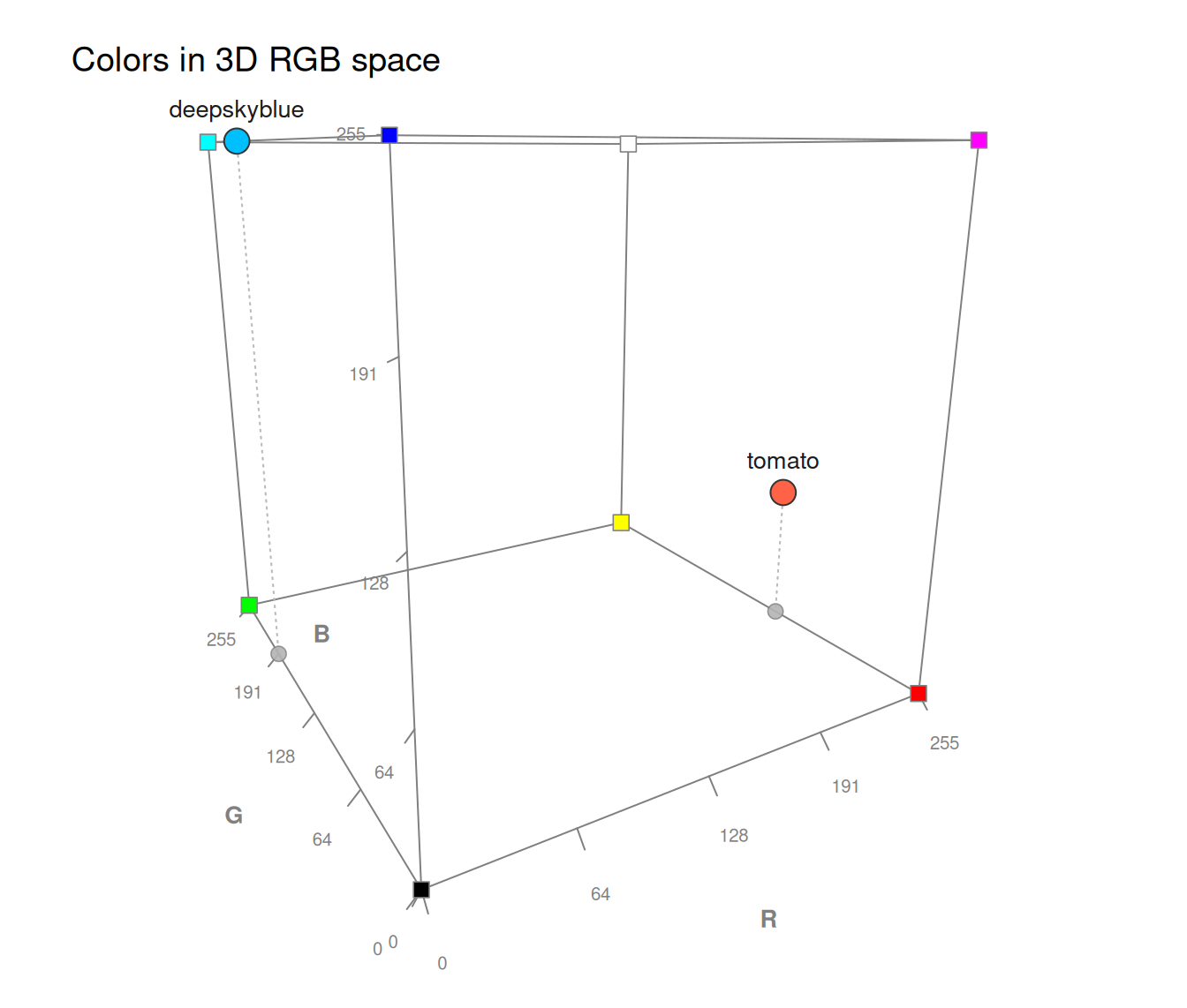
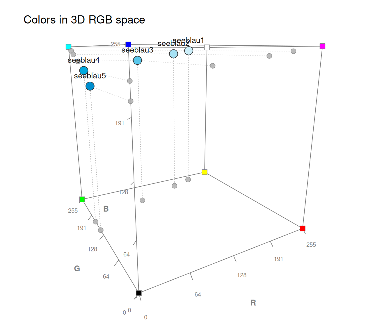
Each shadow is a smaller marker on the corresponding face, linked to its point by a dotted connector. As a projection drops one color channel, a shadow also shows the color with that primary removed. Default: shadows = "none".

col_shadow

Color of the shadow markers. Default: col_shadow = grey(.70, .9) (a neutral grey).

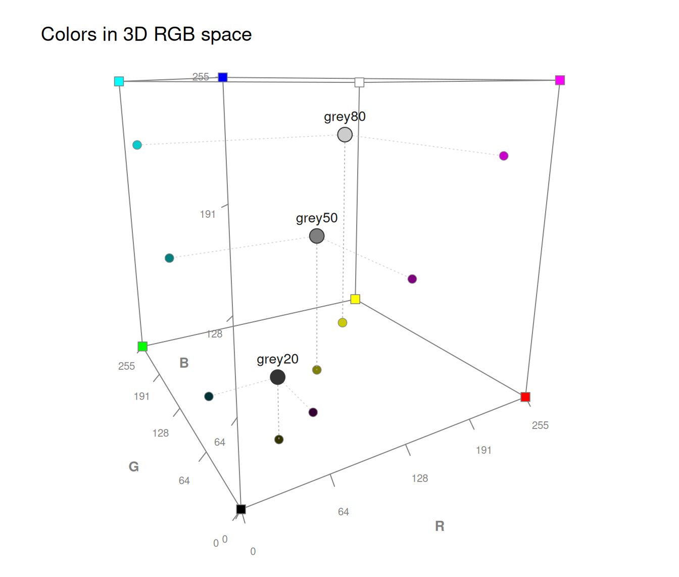
Setting col_shadow = NA shows each shadow in its own projected color. Projecting a point onto a face sets the one color channel perpendicular to that face (i.e., the RGB axis not spanned by the face's plane) to zero: a "floor" shadow sets B = 0, a "back" shadow sets G = 0, and a "side" shadow sets R = 0 (see shadows). As one channel is dropped, a projected shadow color thus systematically differs from its source color: e.g., "violet" (238, 130, 238) casts an orange (238, 130, 0) floor shadow, a magenta (238, 0, 238) back shadow, and a blue (0, 130, 238) side shadow.

show_corners

Boolean option to mark the 8 corners of the cube by points in their corresponding colors (i.e., black, white, and the 6 primary/secondary colors RGB/CMY). Default: show_corners = TRUE.

col_cube

Color for the edges and axes of the cube. Default: col_cube = grey(.50, 1).

grid

Boolean convenience switch to enable a default reference-grid combination (akin to the grid of seecol). grid = TRUE turns on the inner/volume grid (grid_inner = TRUE), which in turn draws the face grid on all 6 faces (grid_faces = "all", so the interior lines end on the faces), at the default spacing (grid_at); grid = FALSE (default) shows no grid. For finer control, set grid_faces, grid_inner, and grid_at directly. Default: grid = FALSE.

grid_faces

Draw reference grid lines on the cube's faces, to ease judging a point's 3D location. Options are:

FALSE: Show no face grid (default);
"base": Grid on the 3 faces meeting at the black corner (floor + 2 near walls);
"all": Grid on all 6 faces (a full box grid).

Line positions are set by grid_at. When grid_inner is enabled, grid_faces defaults to "all" (so the interior lines terminate on the faces), unless set explicitly. Default: grid_faces = FALSE.

grid_inner

Boolean to draw reference grid lines across the cube's volume (interior lines connecting opposite faces: front-to-back, top-to-bottom, and left-to-right), as a 3D orientation aid. Line positions are set by grid_at; best used sparsely (small grid_at), as each position adds many interior lines. (Enabling this also sets grid_faces = "all" by default; see above.) Default: grid_inner = FALSE.

grid_at

Positioning of the grid lines (for grid_faces and grid_inner) along each axis. Options are:

an integer k: Dissect each axis into k equal sub-sections (e.g., 2 = halves/mid-point (default), 3 = thirds, 4 = quarters);
"ticks": At the current axis-tick positions (see n_ticks);
a numeric vector: Use custom positions (in 0:255).

(The endpoints 0 and 255 are always omitted, as they are the cube's edges.) Default: grid_at = 2 (sparse).

col_grid

Color of the face grid lines (grid_faces). Default: col_grid = grey(.60, .60) (a thin, transparent, darker grey).

col_grid_inner

Color of the inner (volume) grid lines (grid_inner). Default: col_grid_inner = grey(.80, .50) (a thin, transparent, lighter grey) — lighter than col_grid, so the face grid reads as the stronger reference.

axis_labels

Titles for the 3 cube axes (R, G, and B). Options are:

a character vector of length\ 3: use these as axis titles;
"short" (or "rgb"): use c("R", "G", "B") (default);
"long": use c("Red", "Green", "Blue");
NA (or "no"): show no axis titles.

Default: axis_labels = c("R", "G", "B").

axis_ticks

Draw tick marks and numeric value labels (in range 0 to 255) along the 3 cube axes? Either a Boolean value, or a numeric vector specifying custom tick positions (in 0:255). Default: axis_ticks = TRUE.

n_ticks

Number of (equally spaced) ticks per axis (only used when axis_ticks = TRUE). Default: n_ticks = 5 (i.e., ticks at 0, 64, 128, 191, 255).

cex_axis

Scaling factor for axis titles and tick values. Default: cex_axis = NA (i.e., use cex_lbl).

labels

Type(s) of labels for the points. One or more of the following label types may be specified (and are shown on separate lines when combined):

"names": show the names of x (or the color values, if no names are available);
"rgb": show each point's RGB triplet (as (R, G, B));
"hex": show each point's HEX value (e.g., "#59C7EB").

Thus, labels = c("names", "rgb", "hex") shows all 3 representations of each color in the same cube. Setting labels = NA (or "no") shows no labels, and passing a character vector (of custom labels) shows these labels instead. Default: labels = "names".

theta

Horizontal rotation angle (azimuth, used by persp). Default: theta = -30.

phi

Vertical rotation angle (colatitude, used by persp). Default: phi = 15.

main

Main plot title. Default: main = "Colors in 3D RGB space".

cex_lbl

Scaling factor for text labels (axes, titles, point labels). Default: cex_lbl = .85.

...

Other (graphical) parameters passed to persp (e.g., d, expand, shade).

Value

A projection matrix (of class returned by persp) that maps 3D coordinates to the 2D plotting plane (returned invisibly).

Details

Each color is converted into its RGB coordinates (via col2rgb) and shown as a point at the corresponding location in the color cube. Points are filled with the color they represent, so that the location of a point in the cube illustrates the additive composition of its color from the three primary colors (Red, Green, and Blue).

plot_cube uses base graphics (i.e., persp and trans3d) and requires no additional package dependencies.

Examples

# A. Basics: ------ 

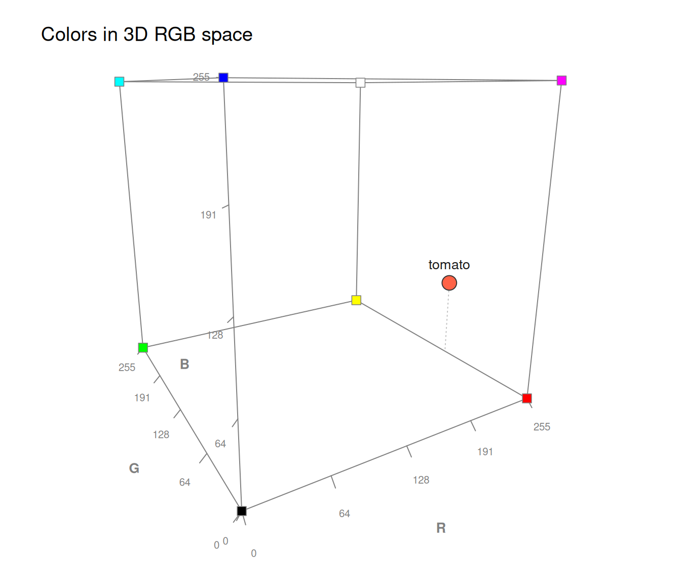
plot_cube("tomato")                        # a single color

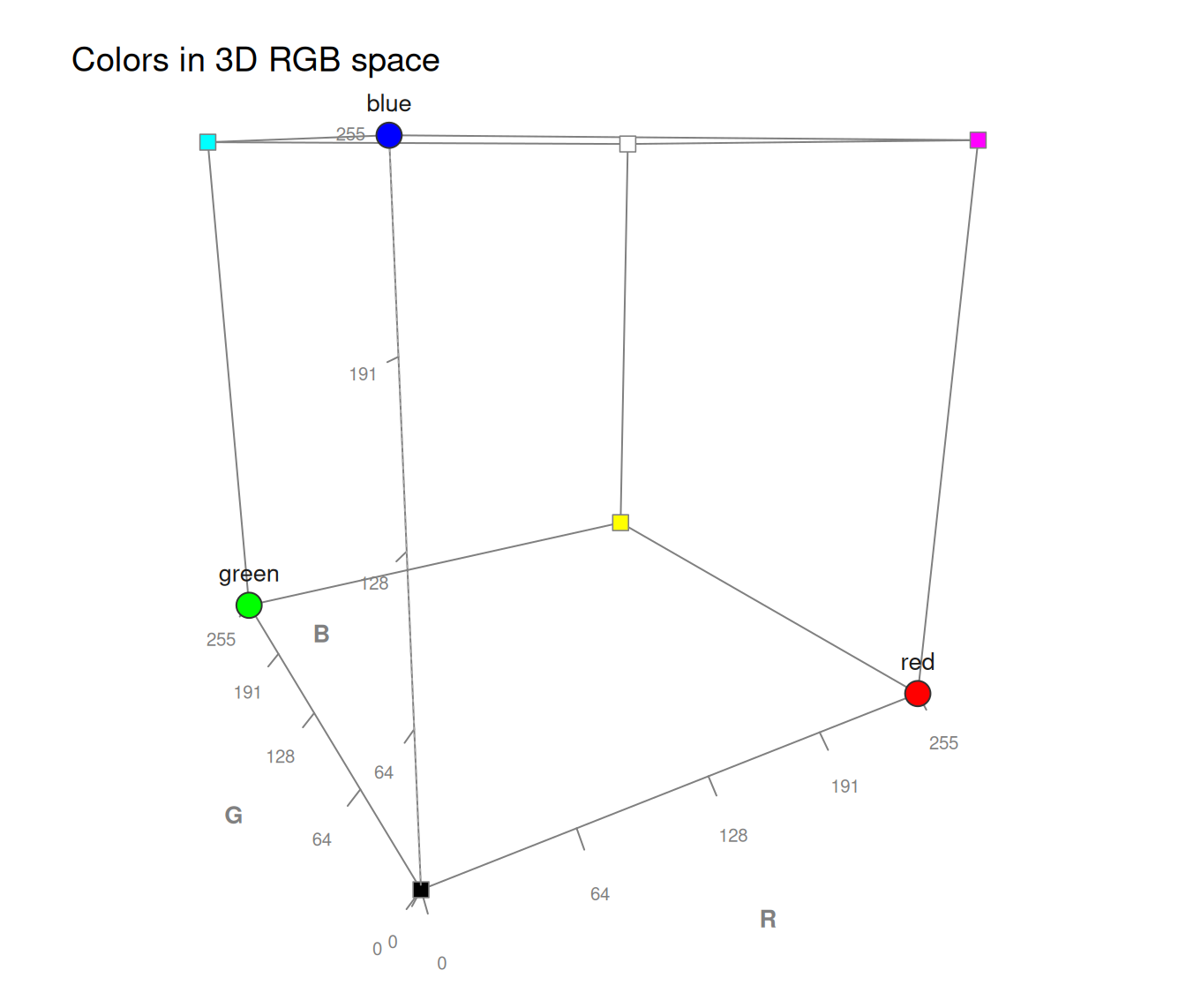
plot_cube(c("red", "green", "blue"))       # primary RGB colors

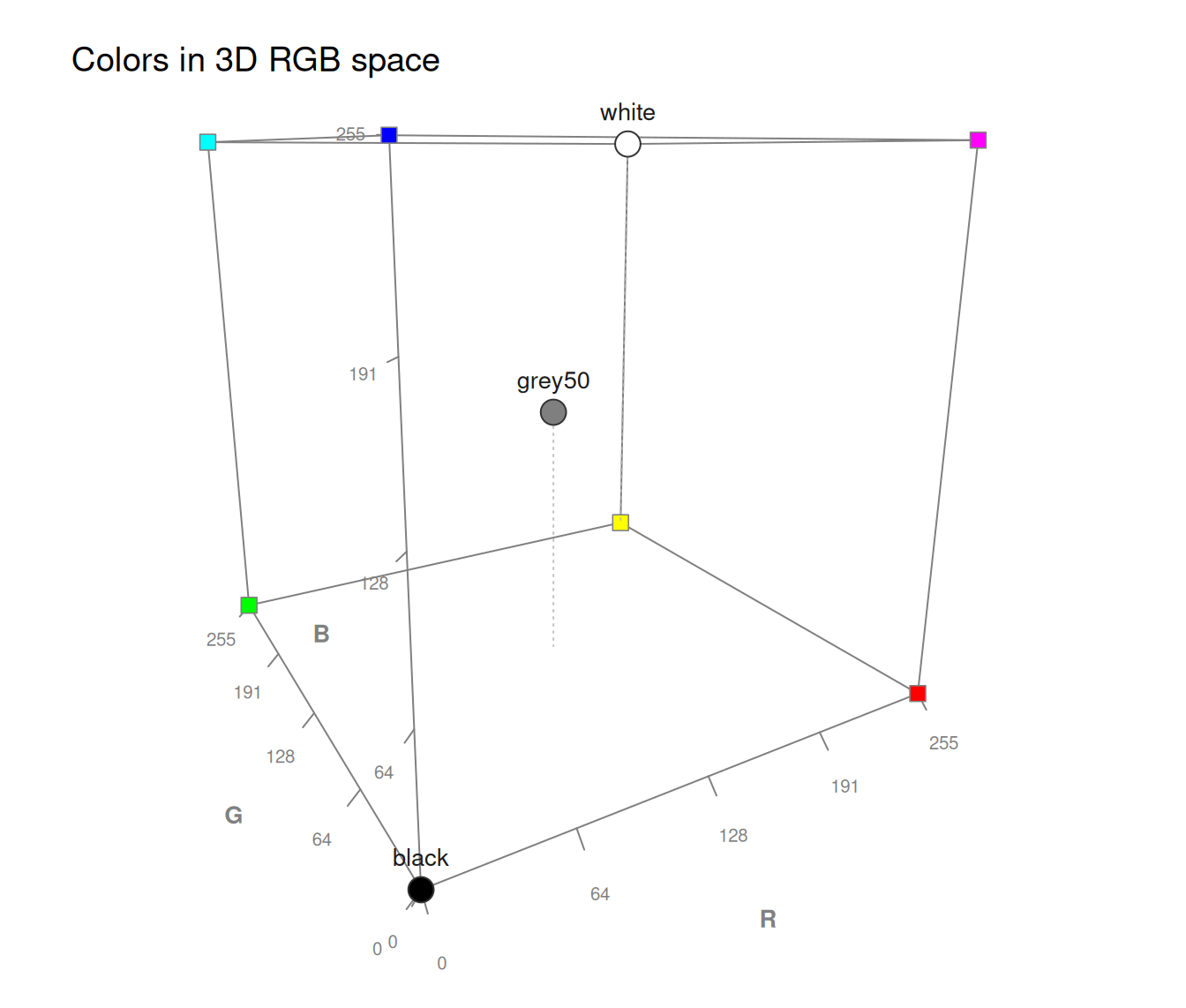
plot_cube(c("black", "grey50", "white"))   # grey diagonal


# Using unikn colors:
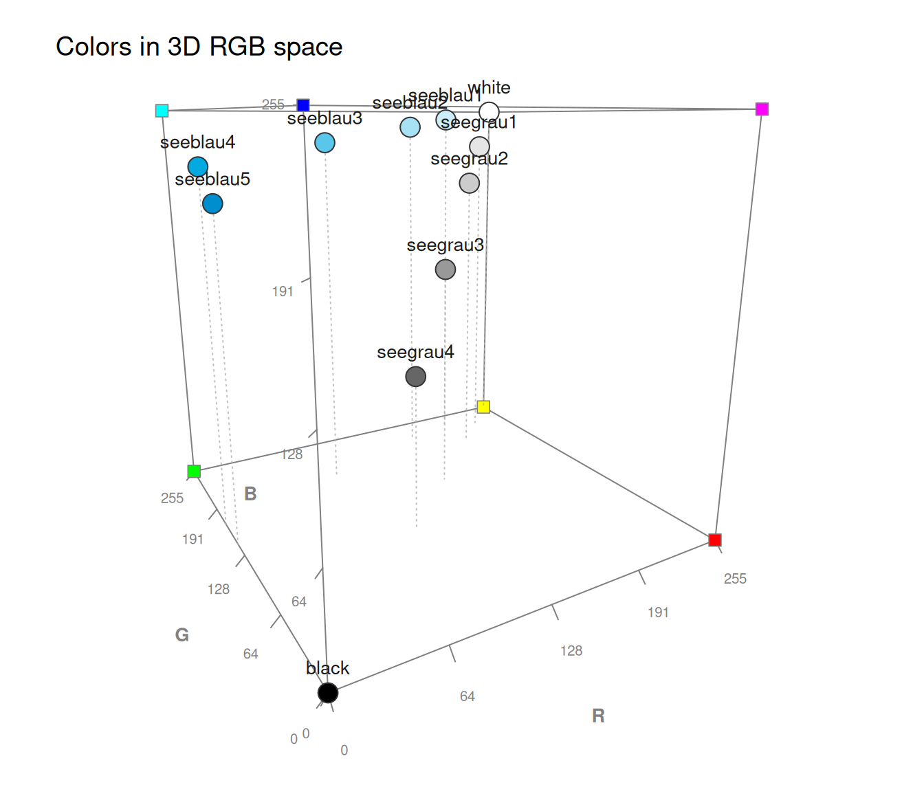
plot_cube(pal_unikn)       # a bi-polar color palette

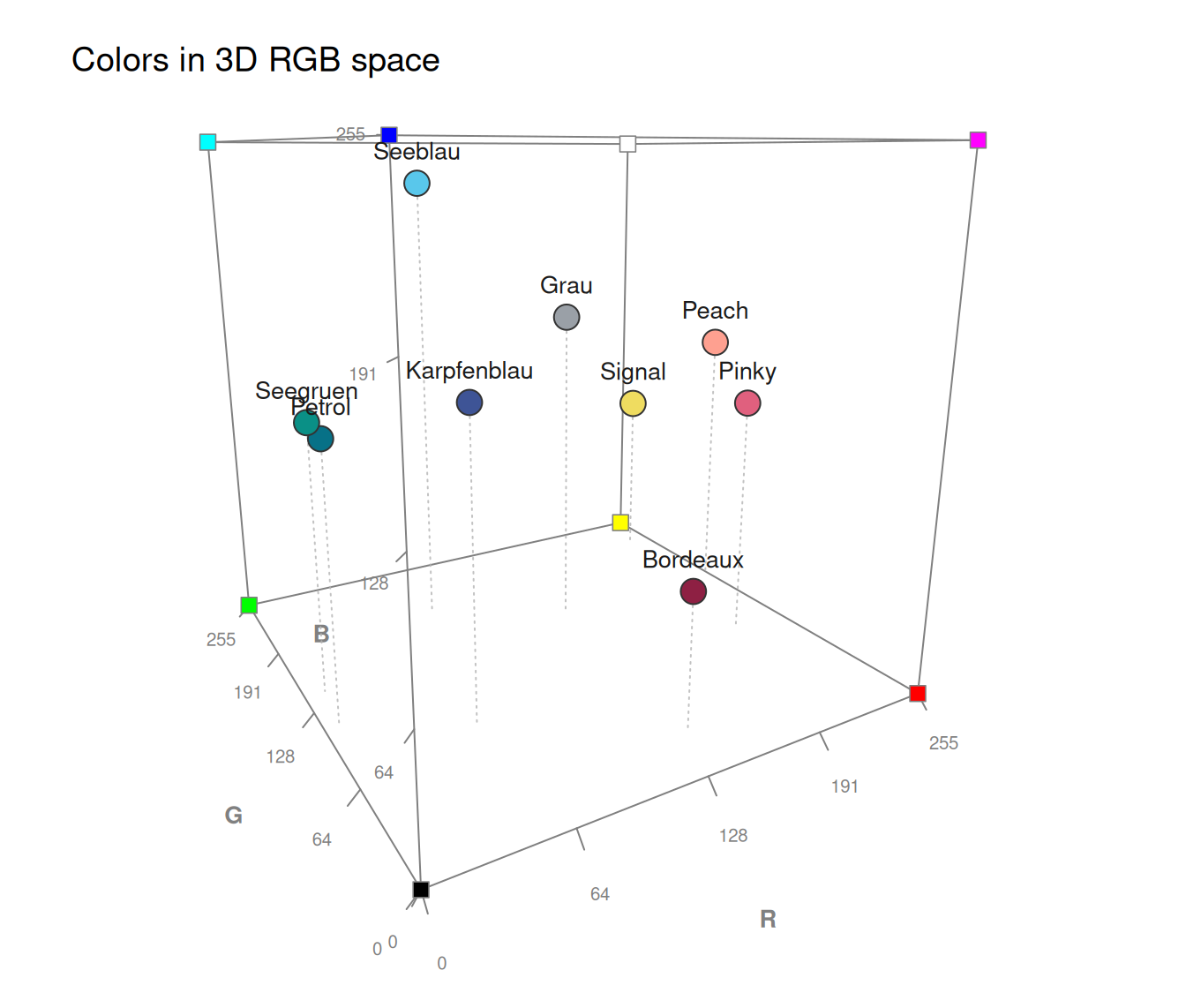
plot_cube(pal_unikn_pref)  # a categorical color palette


# Reduced color options:
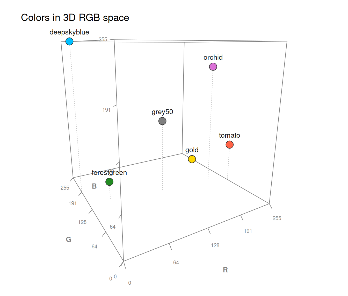
col_mix <- c("grey50", "deepskyblue", "forestgreen", "gold", "orchid", "tomato")
plot_cube(col_mix, show_corners = FALSE)    # hide corner colors

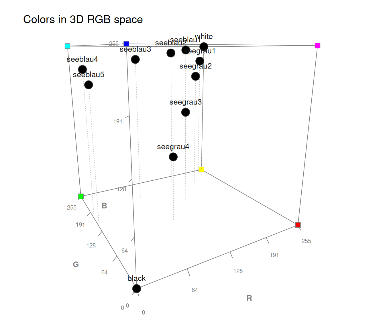
plot_cube(pal_unikn, col_points = "black")  # all points in 1 color


# Labeling points (by names, RGB or HEX values, or combinations):
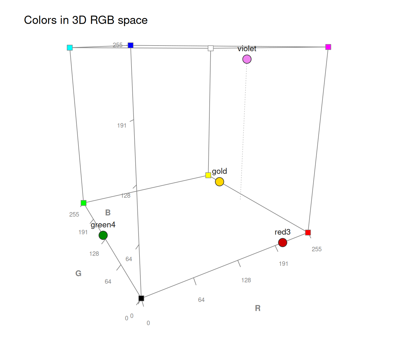
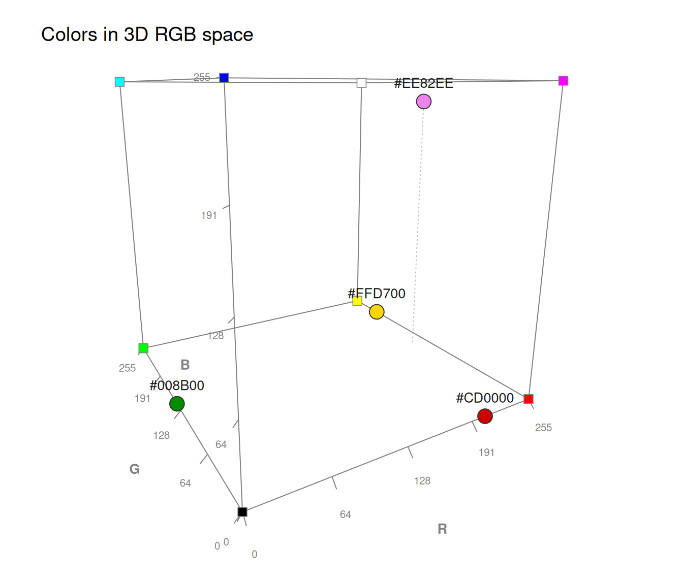
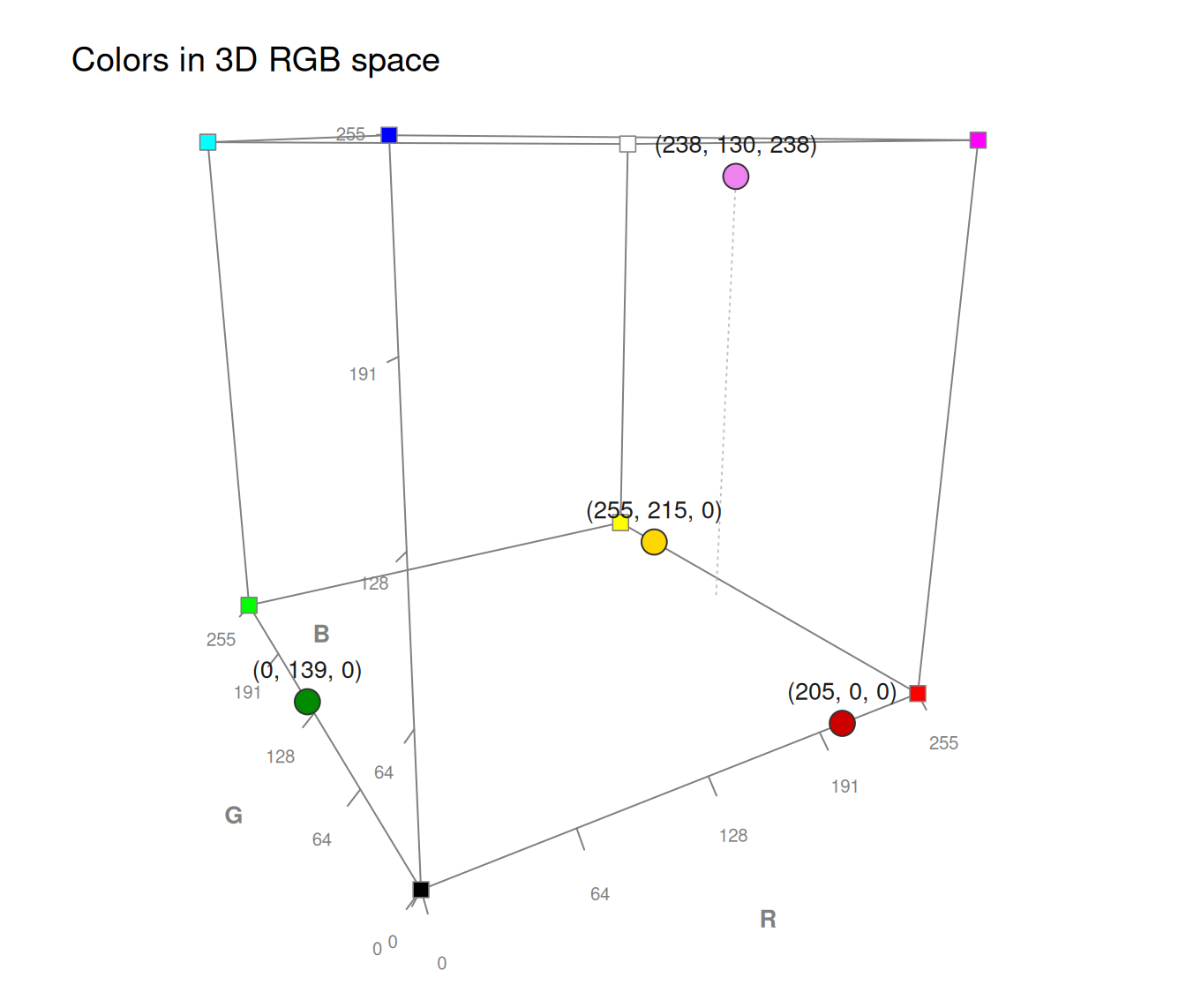
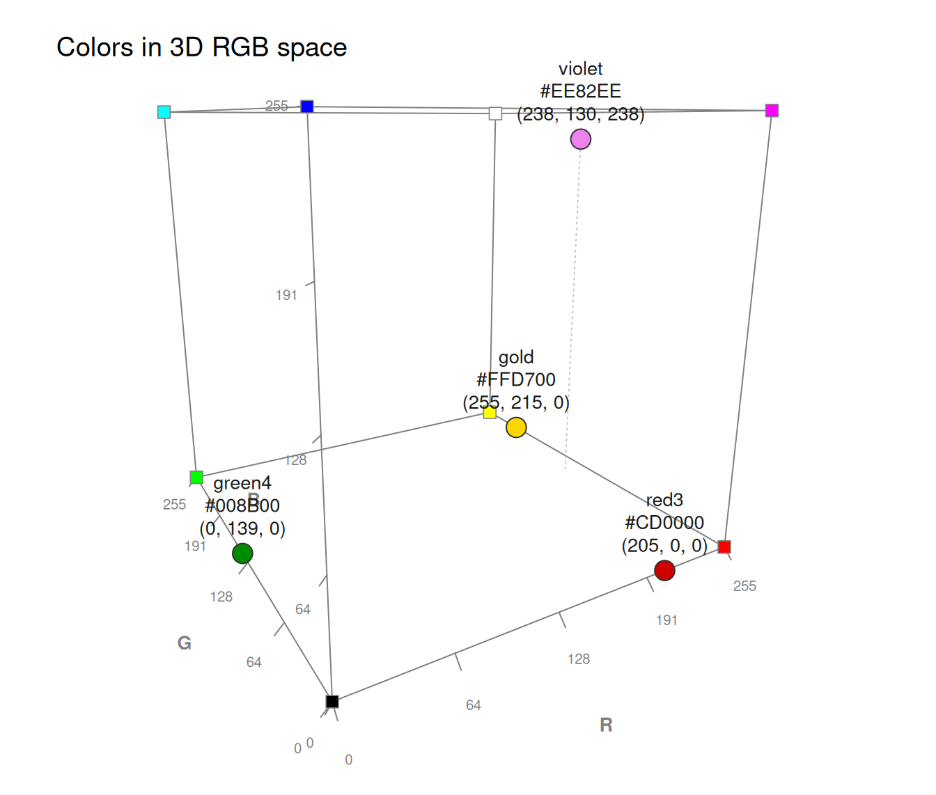
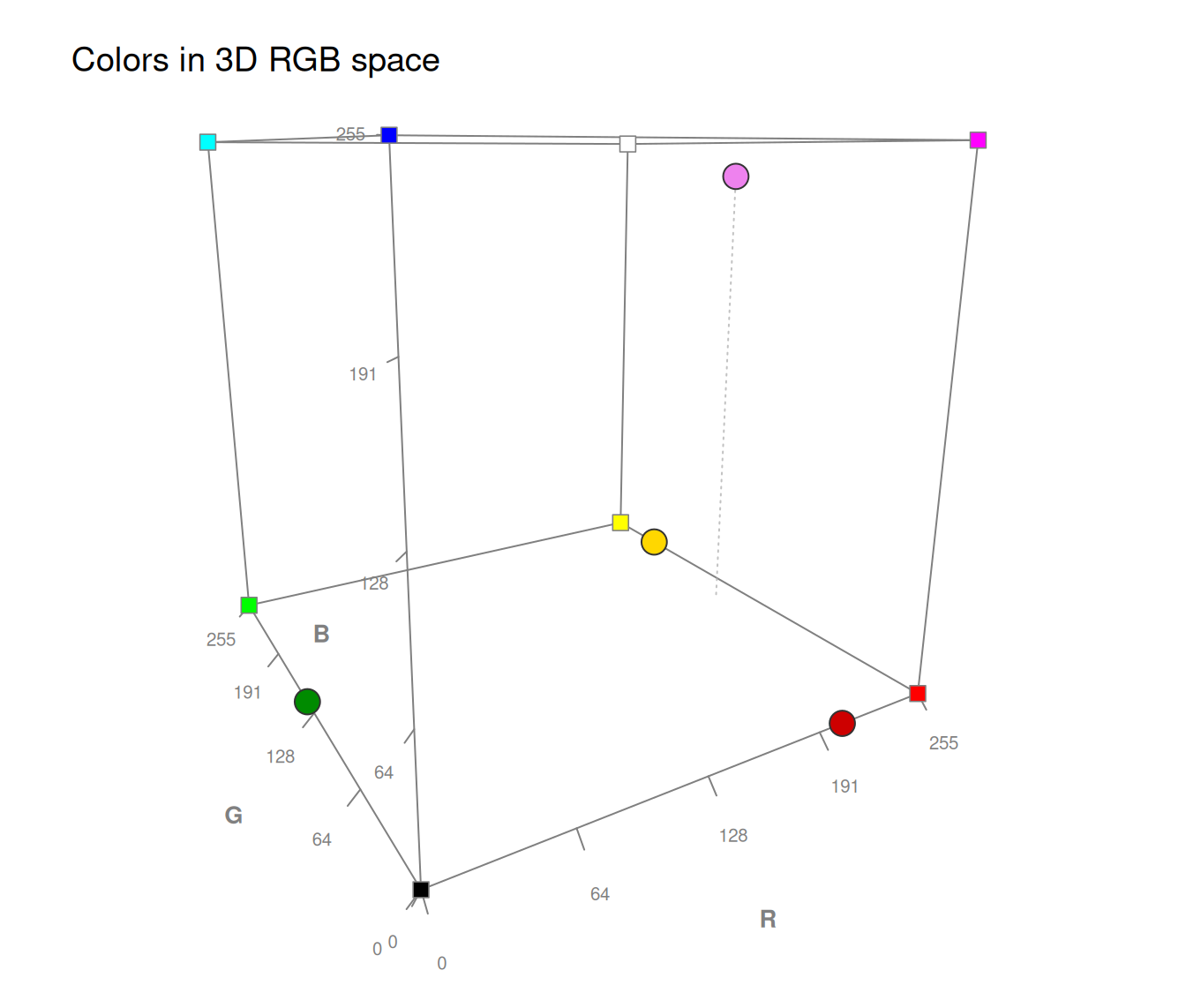
col_4 <- c("red3", "green4", "gold", "violet")
plot_cube(col_4)                                     # names (default)

plot_cube(col_4, labels = "hex")                     # HEX values

plot_cube(col_4, labels = "rgb")                     # RGB values

plot_cube(col_4, labels = c("names", "hex", "rgb"))  # all 3 types

plot_cube(col_4, labels = "no")                      # no labels


# Connecting points by lines (type = "l" or "b"):
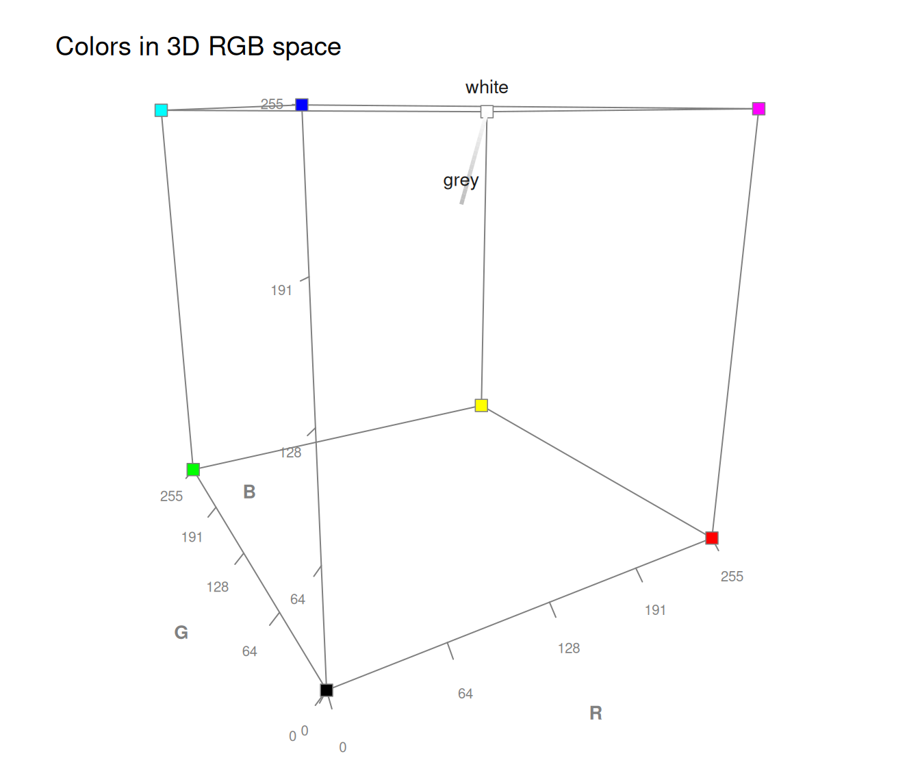
plot_cube(c("grey", "white"), type = "l")          # line (grey diagonal)

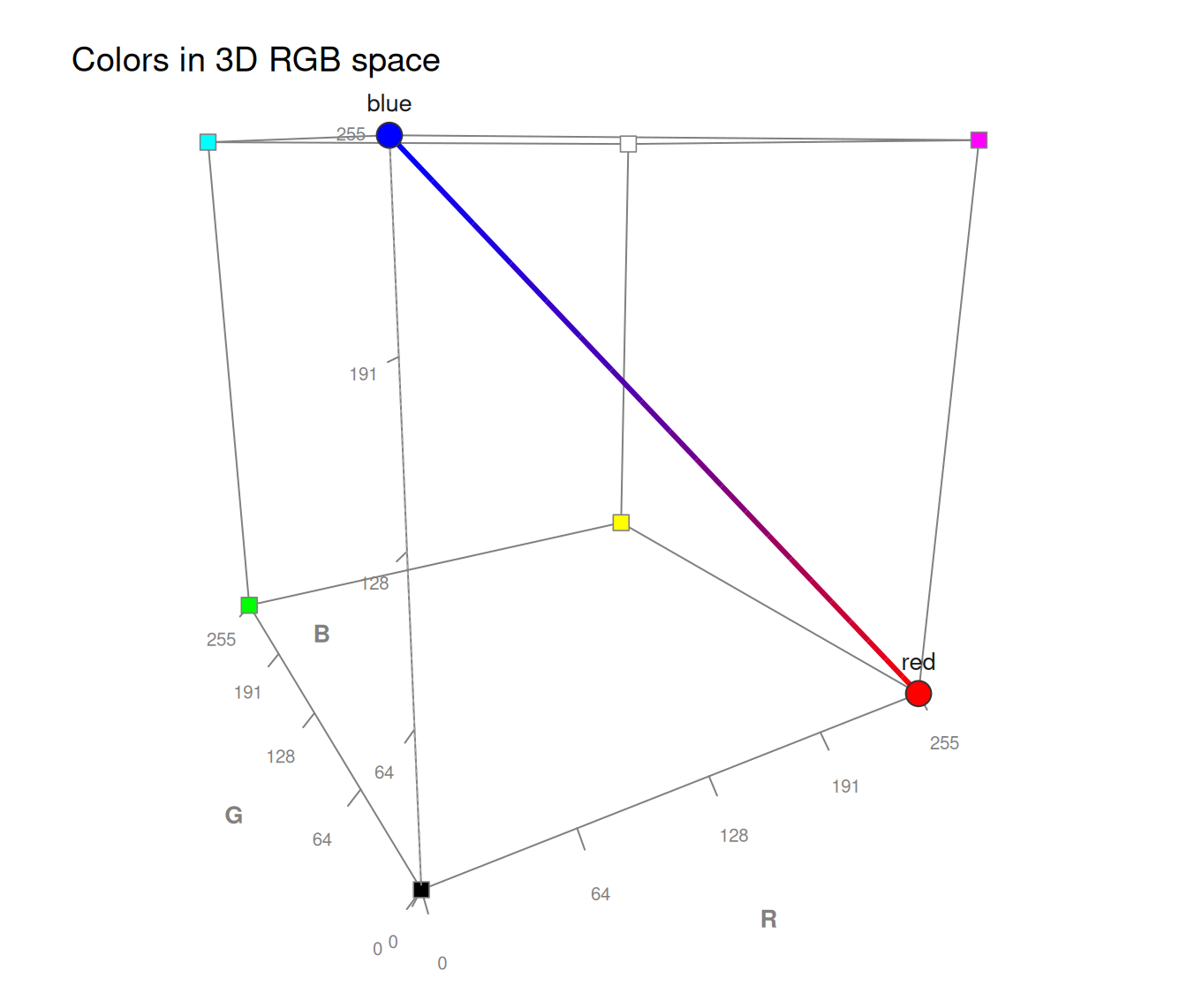
plot_cube(c("red", "blue"), type = "b")            # line with points (red-blue gradient)


# Changing the viewing angle:
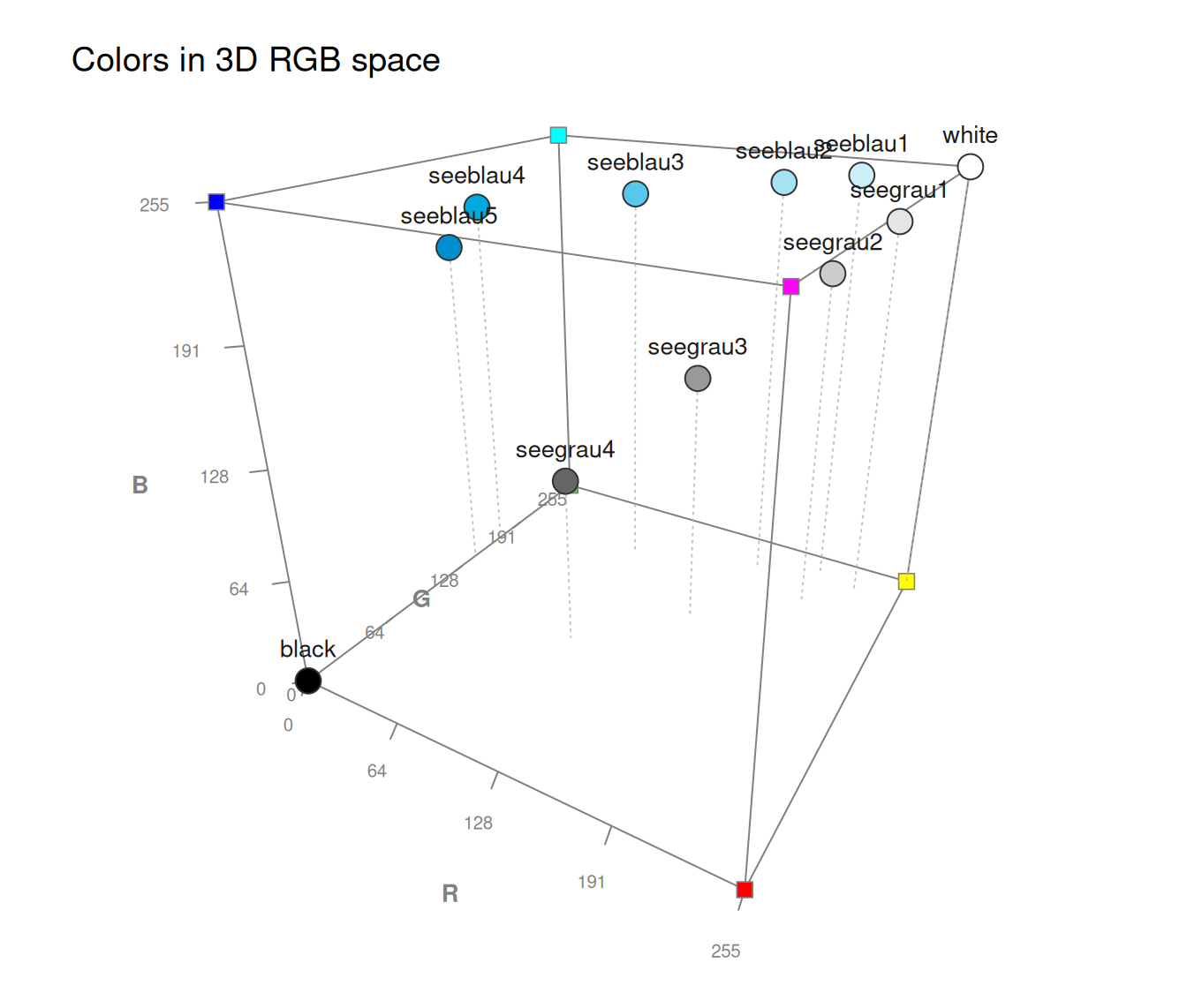
plot_cube(pal_unikn, theta = 30, phi = 25)


# With >2 colors: all pairs (default), disjoint pairs, or a connecting path:
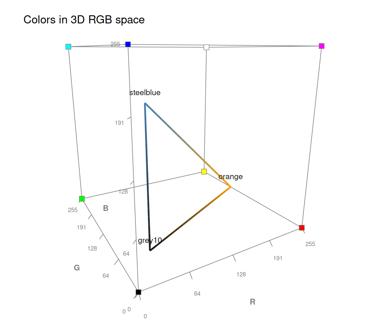
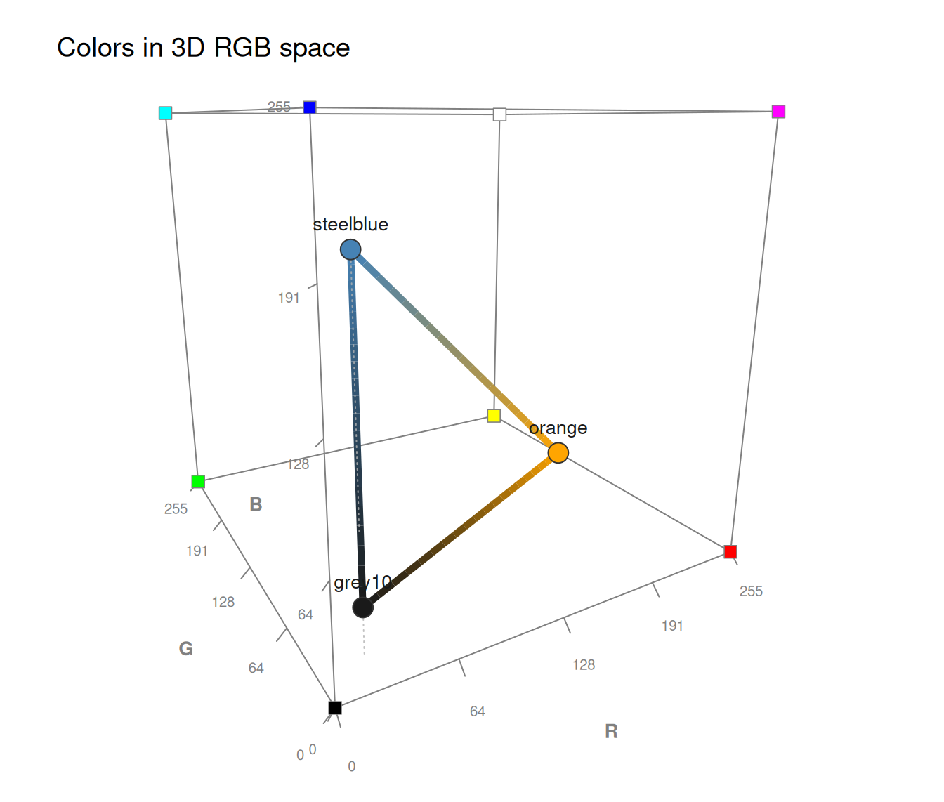
col_3 <- c("grey10", "orange", "steelblue")
plot_cube(col_3, type = "l")                             # all pairs

plot_cube(col_3, type = "b", lwd_line = 5)               # all pairs + points

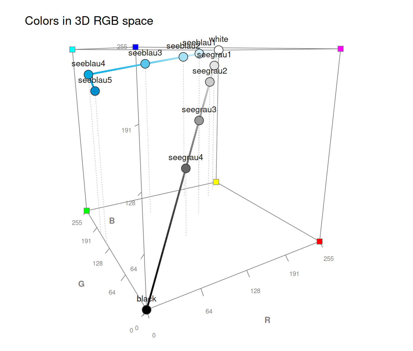
plot_cube(pal_unikn, type = "b", line_connect = "path")  # path (palette order)


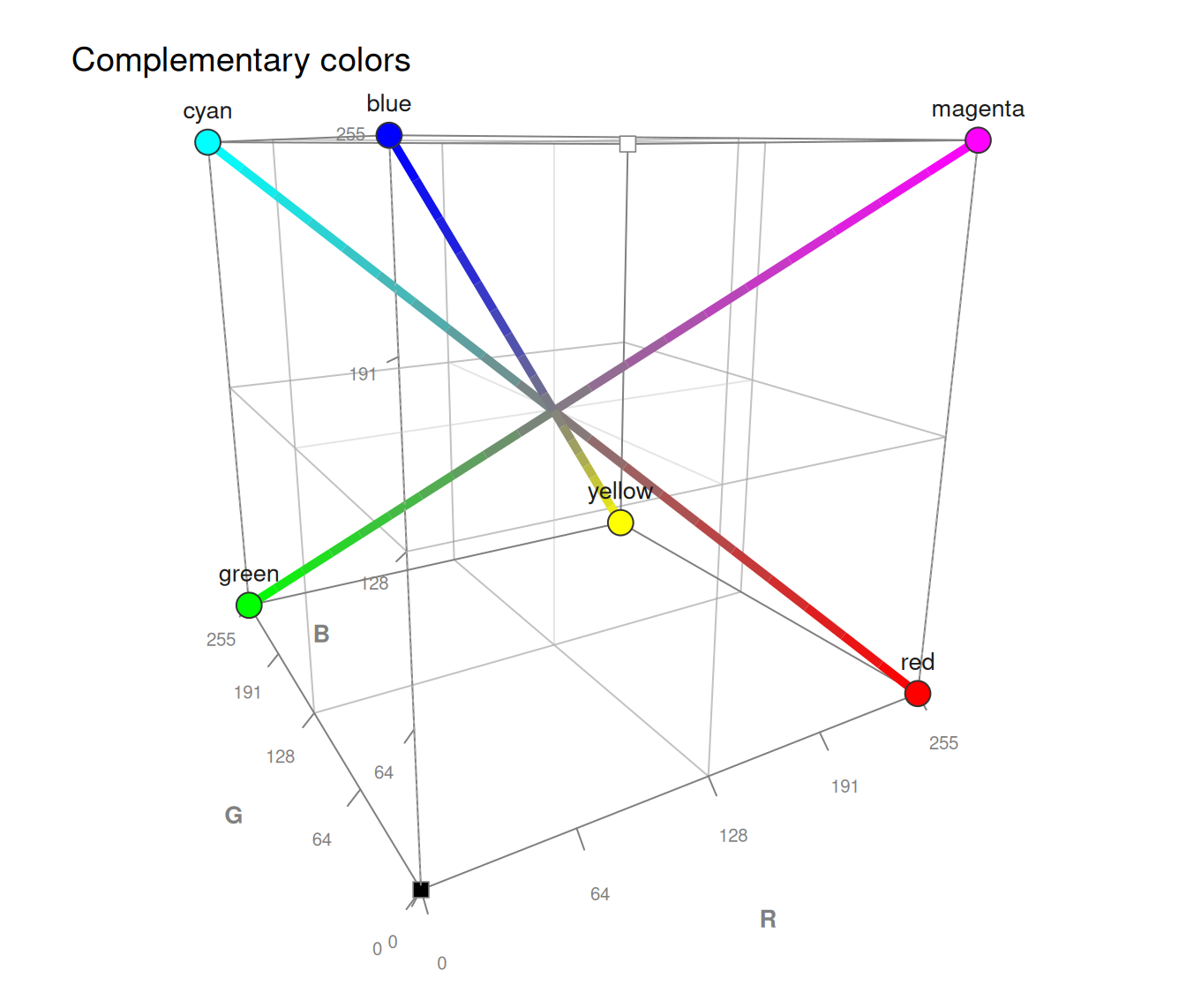
# Using line_connect = "pairs" to link disjoint color pairs, e.g., to show
# the 3 complementary RGB/CMY pairs (each line crosses the grey cube center):
plot_cube(c("red", "cyan", "green", "magenta", "blue", "yellow"), type = "b", 
          line_connect = "pairs", lwd_line = 5, grid = TRUE, main = "Complementary colors")


# Spanning a plane through 3 colors (type = "plane"):
plot_cube(c("red", "green", "blue"), type = "plane")  # gamut of 3 primary RGB colors

plot_cube(c("cyan", "yellow", "magenta"),             # gamut of 3 opposite RGB colors
             type = "plane", labels = c("names", "rgb"))          


# Shadow points (projections onto cube faces):
plot_cube(c("tomato", "deepskyblue"), shadows = "floor")  # on the floor (B = 0)

plot_cube(pal_seeblau, shadows = "all")                   # on all 3 faces

plot_cube(c("grey20", "grey50", "grey80"),                # show shadows in projected colors
          shadows = "all", col_shadow = NA) 

          
# Axis options (titles and value ticks):
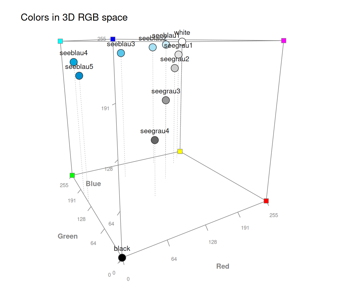
plot_cube(pal_unikn, axis_labels = "long")           # long axis titles

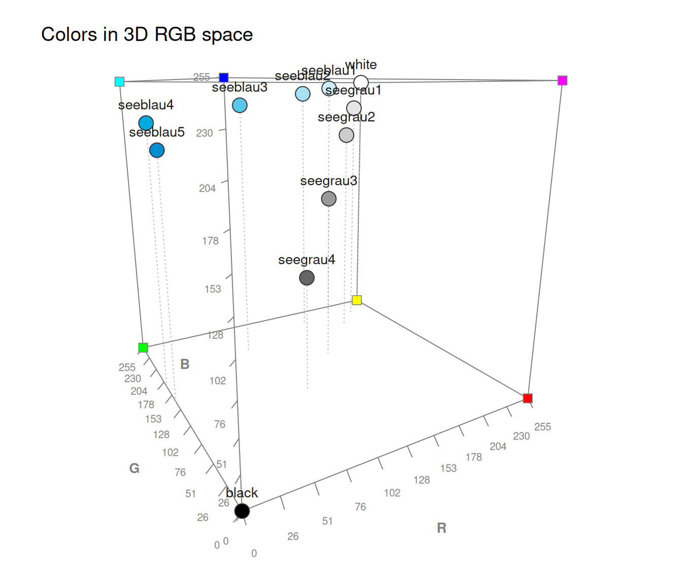
plot_cube(pal_unikn, n_ticks = 11)                   # finer axis scale (0, 25.5, ...)

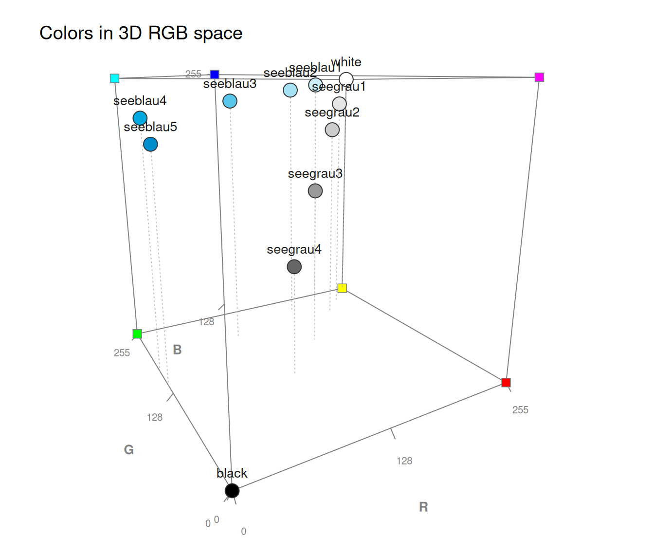
plot_cube(pal_unikn, axis_ticks = c(0, 128, 255))    # custom tick positions

plot_cube(pal_unikn, axis_ticks = FALSE)             # no ticks (titles only)

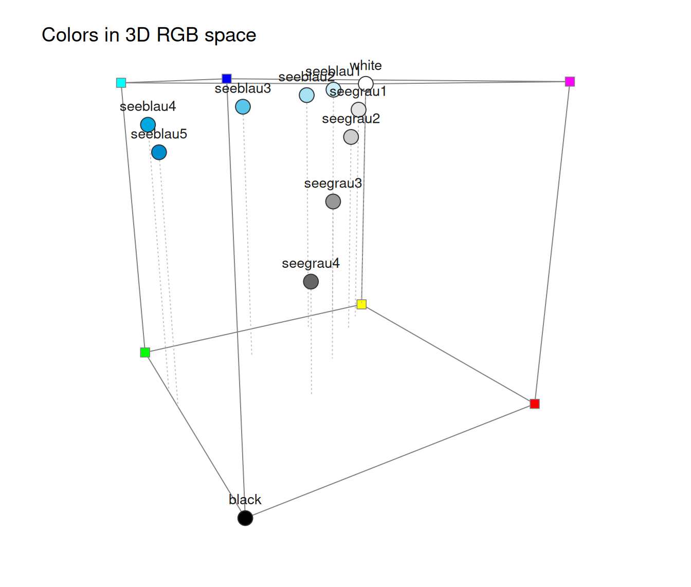
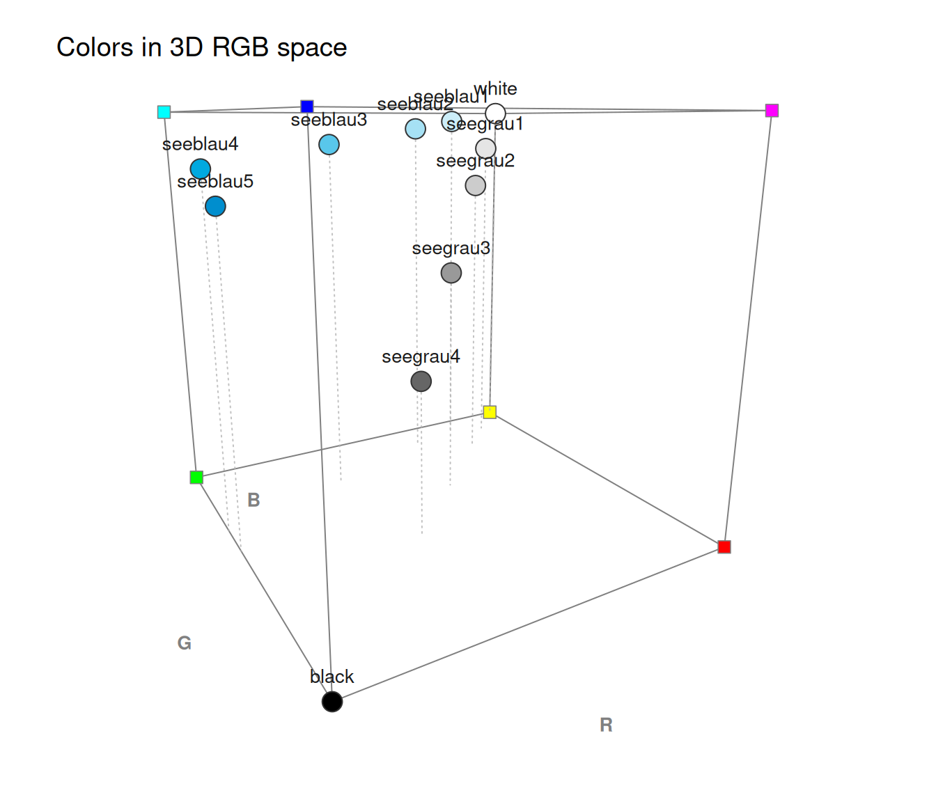plot_cube(pal_unikn, axis_labels = "no", axis_ticks = FALSE)  # bare cube


# Grid options (to aid judging 3D locations): 
# Both reference grids improve orientation, but only when used sparsely.

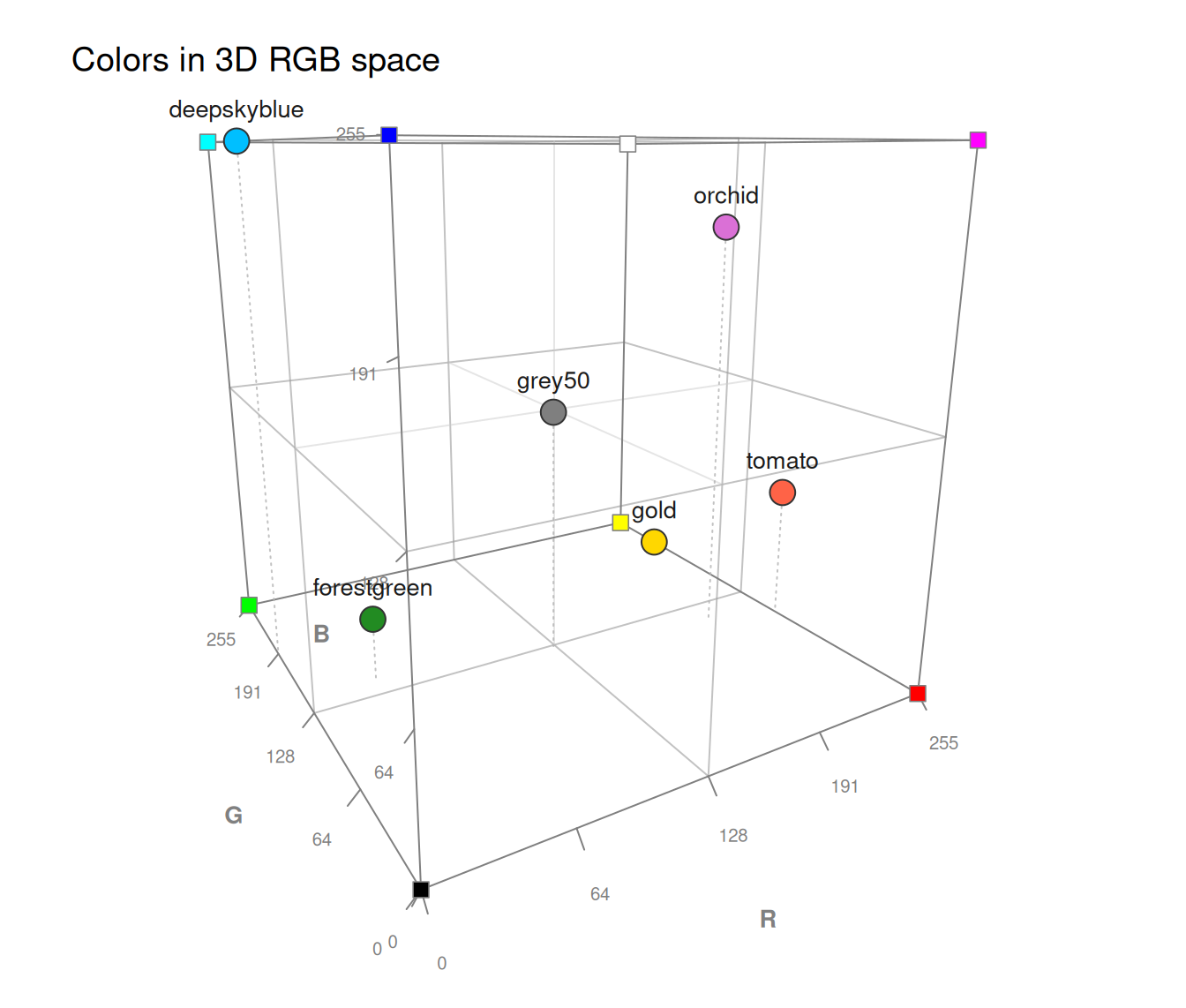
# a. Default of grid = TRUE (splits cube into octants): 
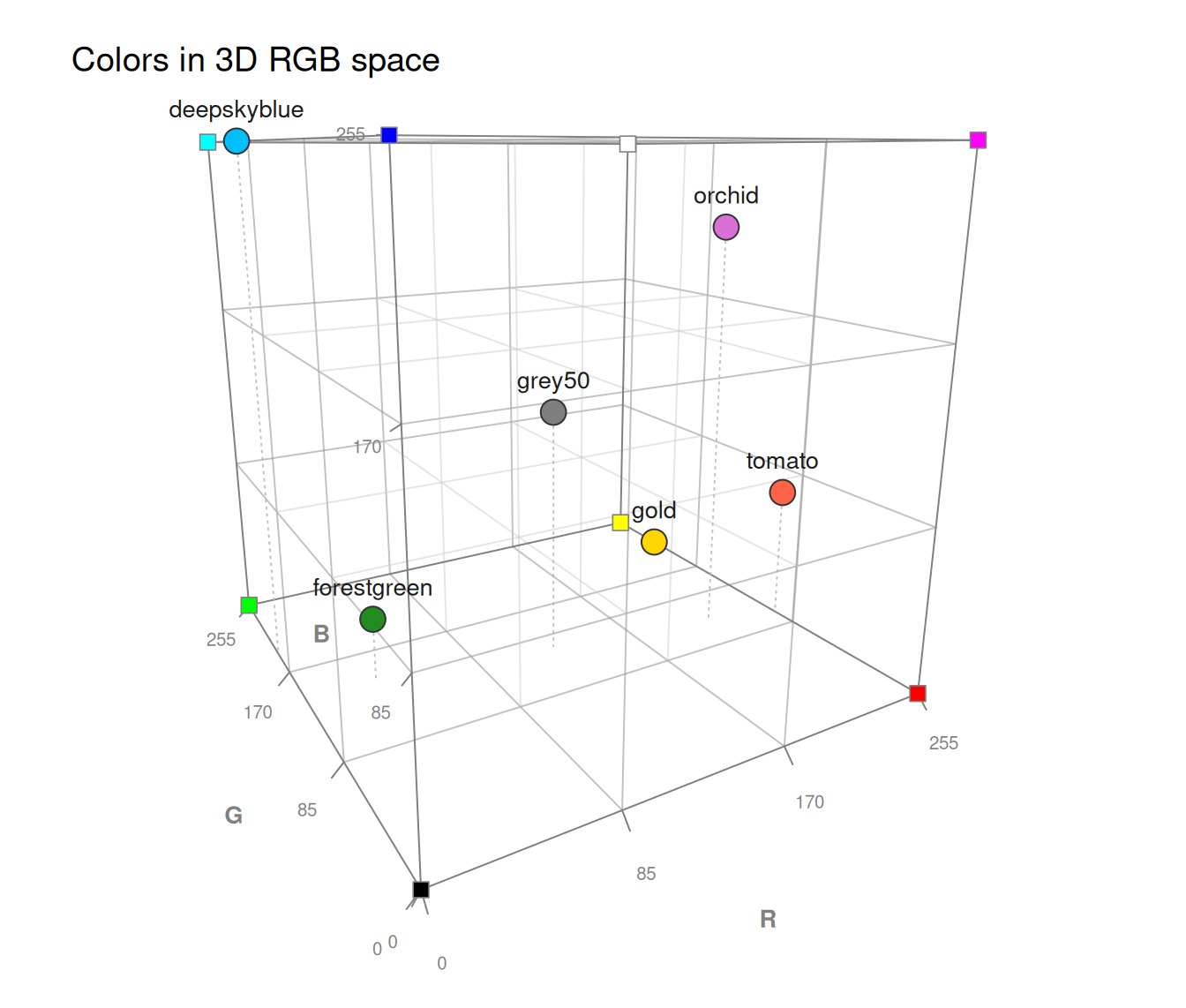
col_mix <- c("grey50", "deepskyblue", "forestgreen", "gold", "orchid", "tomato")
plot_cube(col_mix, grid = TRUE)


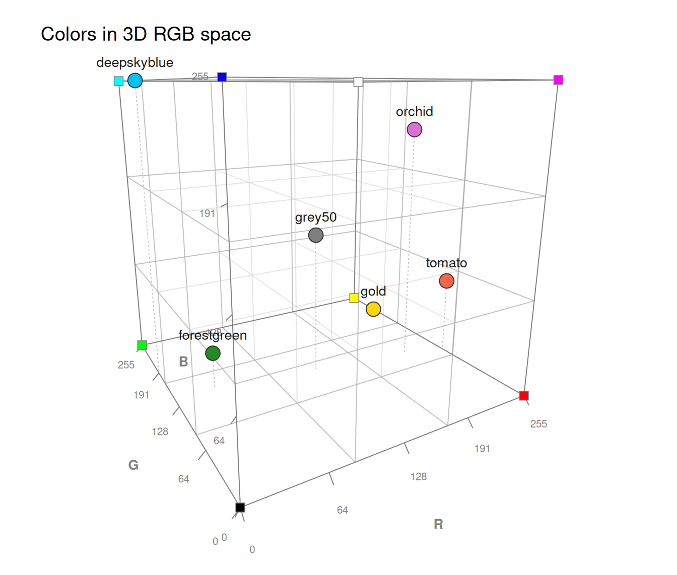
# b. Both grids at thirds (more structure, but quickly gets dense): 
plot_cube(col_mix, grid = TRUE, grid_at = 3)


# c. Both grids at rare axis ticks (to align grid with tick labels):
plot_cube(col_mix, grid = TRUE, grid_at = "ticks", n_ticks = 4)


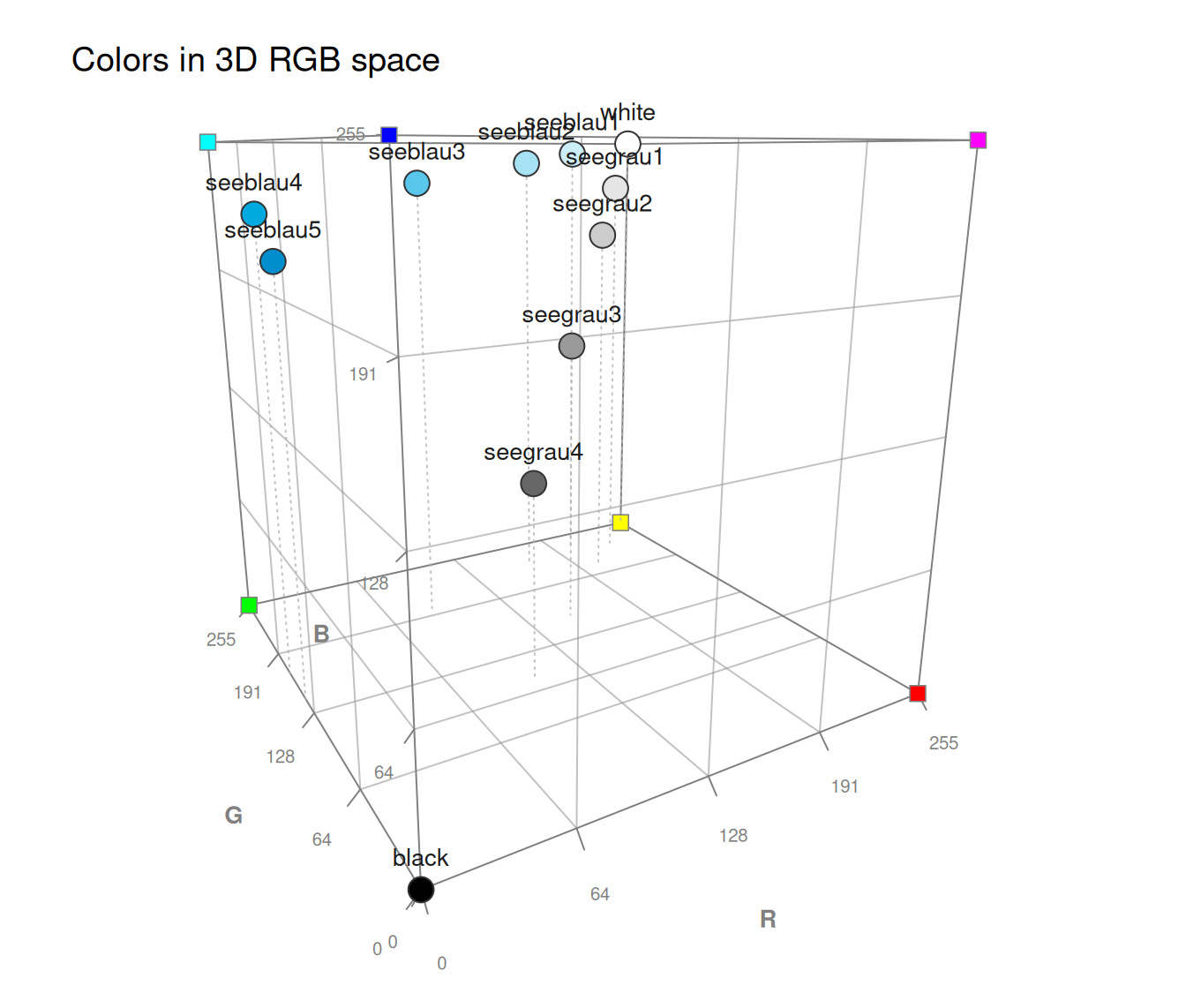
# d. Face grid only (often suffices, as inner grid may not be needed):
plot_cube(pal_unikn, grid_faces = "base", n_ticks = 5, grid_at = "ticks")



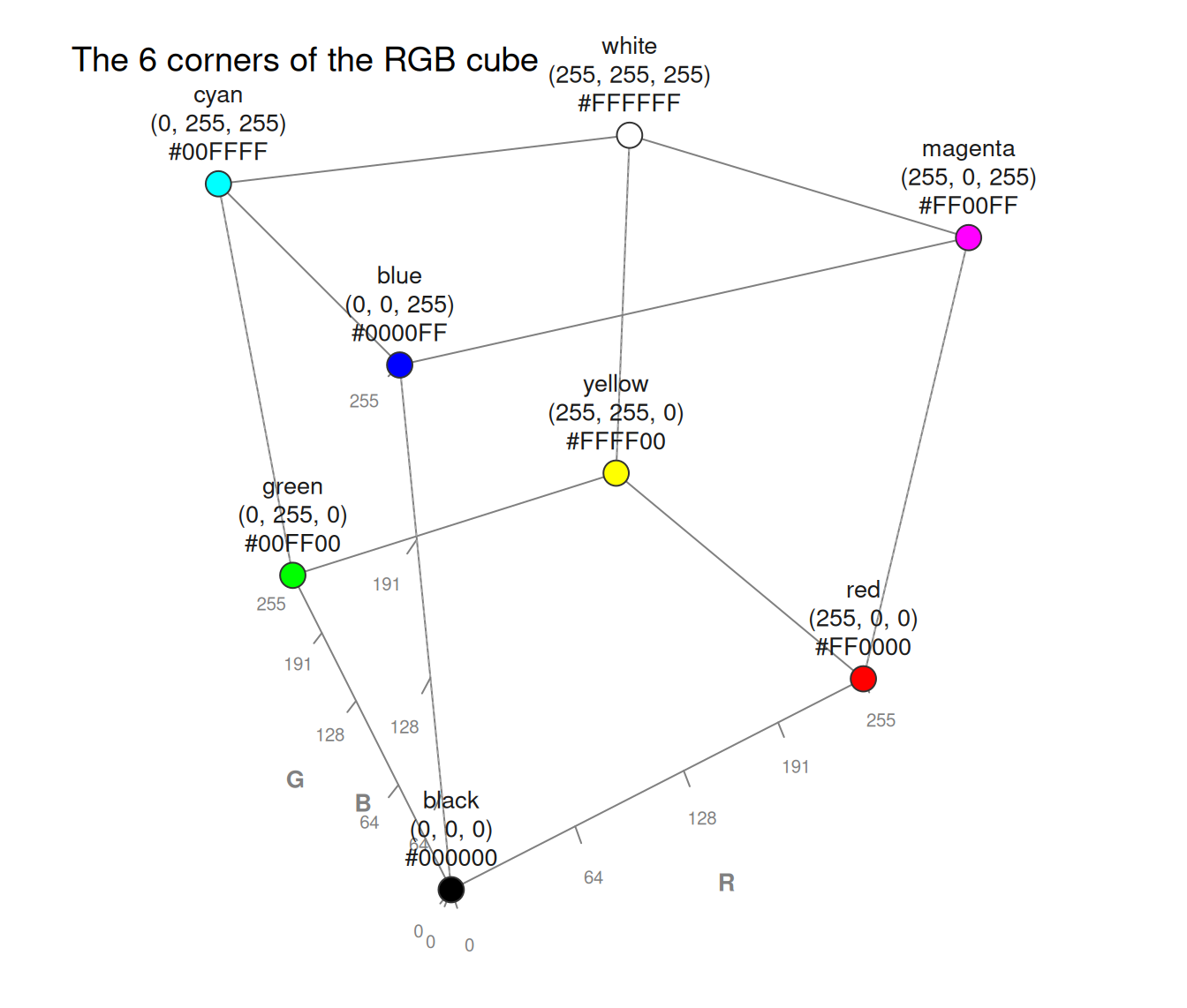
# B. Basic demonstrations of the 3D color cube (RGB/CMY): ------

# 1. The 8 color corners of the RGB cube (b/w + RGB + CMY):
col_8 <- c("black", "white", "red", "cyan", "blue", "yellow", "green", "magenta")
plot_cube(col_8, theta = -30, phi = 30, labels = c("names", "rgb", "hex"),
          main = "The 6 corners of the RGB cube")


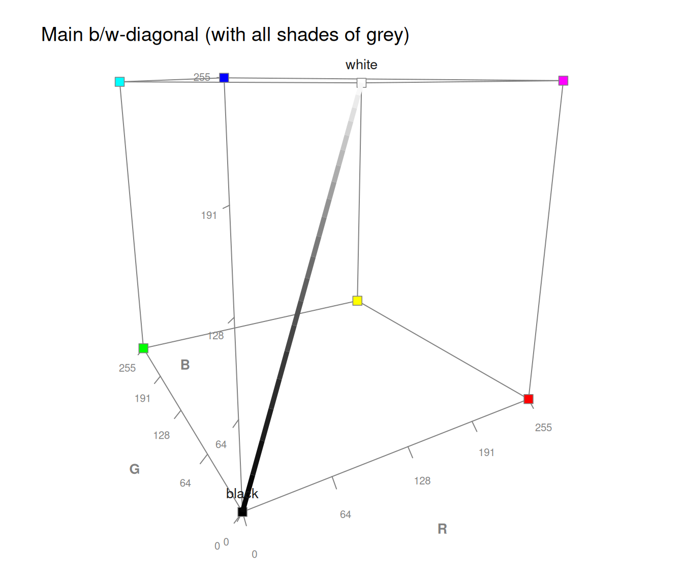
# 2. The main black-grey-white diagonal of the cube (with all shades of grey):
plot_cube(c("black", "white"), type = "l", lwd_line = 5, 
          main = "Main b/w-diagonal (with all shades of grey)")

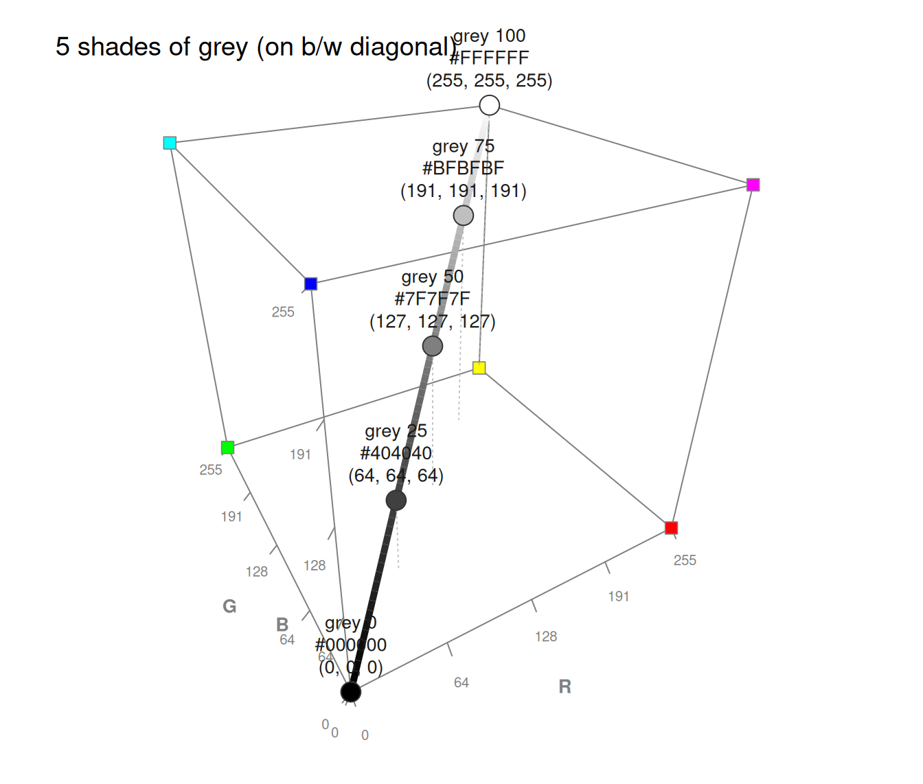
greys <- paste("grey", seq(0, 100, length.out = 5))  # 5 shades of grey (white to black)
plot_cube(greys, type = "b", line_connect = "path", 
          lwd_line = 5, labels = c("names", "hex", "rgb"),
          theta = -30, phi = 30, 
          main = "5 shades of grey (on b/w diagonal)")


# 3. Complementarity of the RGB and CMY color systems:
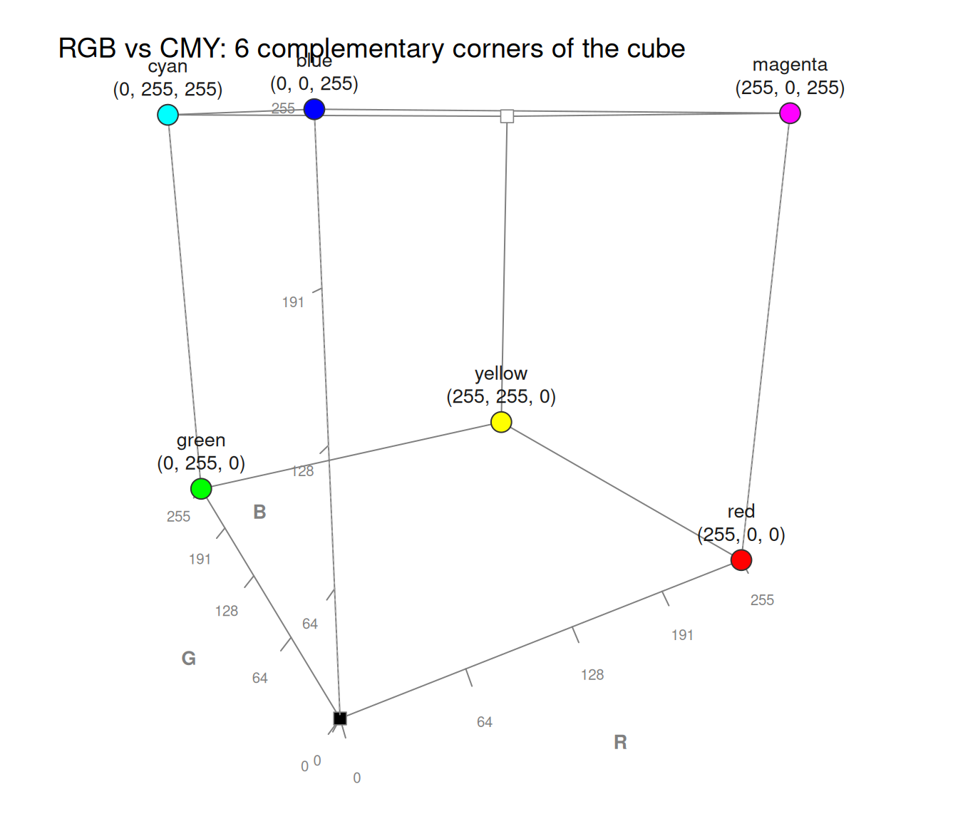
#    Each CMY secondary (cyan, magenta, yellow) is the complement of an RGB
#    primary (red, green, blue): it occupies the opposite corner of the cube,
#    and a color and its complement mix to grey (at the cube's center).

# Show 6 color corners (RGB vs. CMY):
col_6 <- c("red", "cyan", "blue", "yellow", "green", "magenta")
plot_cube(col_6, labels = c("names", "rgb"),
          main = "RGB vs CMY: 6 complementary corners of the cube")

          
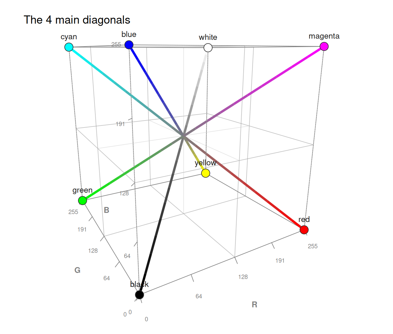
# Show all 4 cube diagonals:
plot_cube(col_8, type = "b", line_connect = "pairs", lwd_line = 4,
          grid = TRUE, main = "The 4 main diagonals")

            
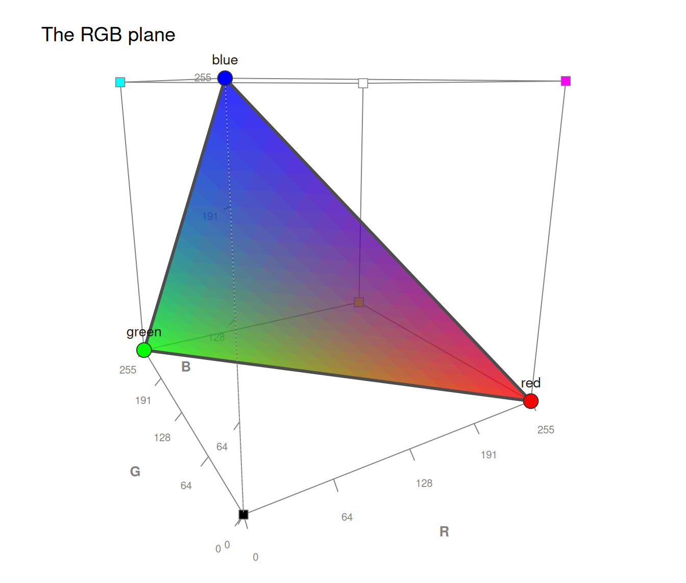
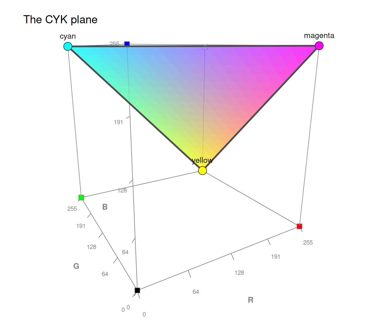
# Show 2 triangular planes:
plot_cube(c("red", "blue", "green"), type = "plane", main = "The RGB plane")

plot_cube(c("cyan", "yellow", "magenta"), type = "plane", main = "The CYK plane")



# C. Illustrating colors and color palettes (unikn): ------

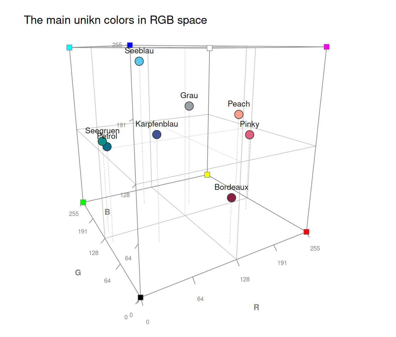
# 0. Collect main unikn colors (as a vector):
col_4 <- c(Seeblau, Pinky, Seegruen, Bordeaux)
col_8 <- c(col_4, Petrol, Karpfenblau, Peach, Grau)

# 1. Main unikn colors as (labeled) points:
plot_cube(col_8, grid = TRUE, main = "The main unikn colors in RGB space")


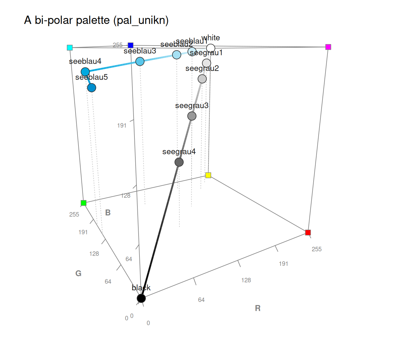
# 2. The default unikn palette (black - Seeblau shades - white) as a path:
plot_cube(pal_unikn, type = "b", line_connect = "path", lwd_line = 3,
          main = "A bi-polar palette (pal_unikn)")

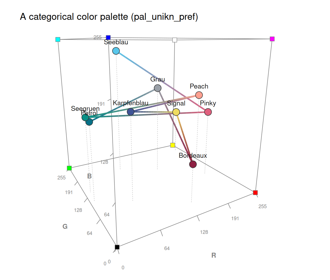
plot_cube(pal_unikn_pref, type = "b", line_connect = "path", lwd_line = 3,
          main = "A categorical color palette (pal_unikn_pref)")

          
# 2. A color palette's shade ramp as a connecting path:
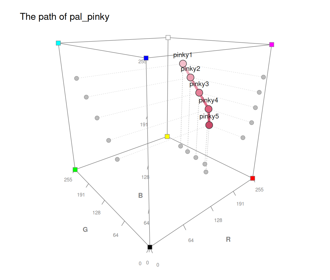
plot_cube(pal_pinky, type = "b", line_connect = "path", lwd_line = 5,
          theta = -40, phi = 20, shadows = "all", main = "The path of pal_pinky")

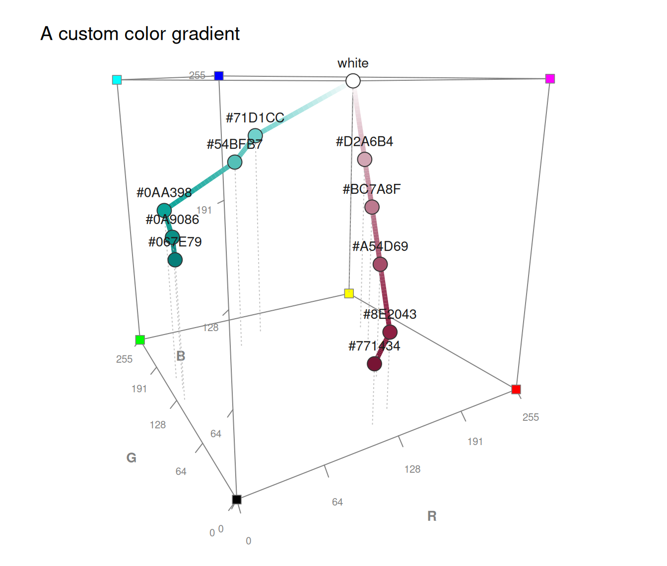
plot_cube(usecol(c(rev(pal_seegruen), "white", pal_bordeaux)), type = "b", 
          line_connect = "path", lwd_line = 5, main = "A custom color gradient")

          
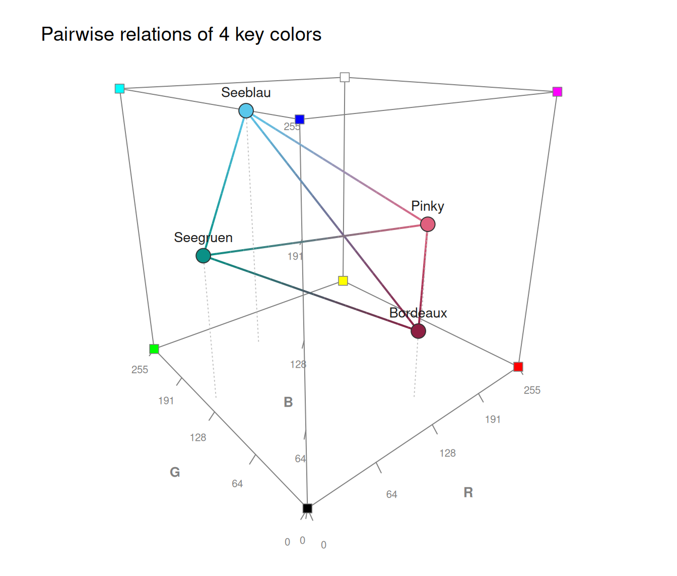
# 4. Pairwise relations among main colors:
plot_cube(col_4, type = "b", lwd_line = 2, theta = -40, phi = 20, 
          main = "Pairwise relations of 4 key colors")


# 5. The gamut (plane) of mixtures spanned by 3 main colors:
plot_cube(c(Seeblau, Pinky, Seegruen), type = "plane",
          theta = 10, phi = 20, main = "Gamut of 3 key colors")